元值

In the last chapter we talked about vector spaces and in the next chapter we will talk about linear transformations across vector spaces, but in this chapter we must focus on a topic that links both topics together, eigenvalues  and eigenvectors .
::在最后一章中,我们谈到矢量空间,在下一章中,我们将谈到矢量空间的线性转变,但在本章中,我们必须着重讨论一个将两个专题联系在一起的主题,即源值和源值。

In this lesson; however, we will focus primarily on eigenvalues. Before I tell you what an eigenvalue is let's look at this basic linear transformation, as a matter of fact let's look back on the example we used in an earlier chapter.
::在此教训中, 但是, 我们主要关注 igenvalues 。 在我告诉你什么是 eigenvalues 之前, 让我们先看看这个基本的线性转变, 事实上, 让我们回顾一下我们在前一章中使用的例子 。

Let  $\begin{align*}T:\mathbb{R}^{2}\longrightarrow\mathbb{R}^{2}\end{align*}$  and define  $\begin{align*}T(\vec{x})=\begin{bmatrix}-5 & -2\\2 & -1\end{bmatrix}\cdot\vec{x}\end{align*}$  where  $\begin{align*}\vec{x} = \begin{bmatrix}x_{1}\\x_{2}\end{bmatrix}\end{align*}$ . Now let's try out some examples for the vector  $\begin{align*}\vec{x}\end{align*}$ .
::让 T: R2R2 并定义 T( x) = [- 5- 22- 1- 1] =\ x = [x1x2] 。 现在让我们尝试一下矢量 x 的一些示例 。

播放段落
•  Let  $\begin{align*}\vec{x} = \begin{bmatrix}1\\0\end{bmatrix} \text{ and then } T(\vec{x}) = \begin{bmatrix}-5\\2\end{bmatrix}\end{align*}$
  ::Let _x=[10] 然后T(%x) =[-52]

播放段落
•   Let  $\begin{align*}\vec{x} = \begin{bmatrix}0\\1\end{bmatrix} \text{ and then } T(\vec{x}) = \begin{bmatrix}-2\\-1\end{bmatrix}\end{align*}$  
  ::Let 'x=[01] 然后T(%x) =[-2- 1]

播放段落
•   Let  $\begin{align*}\vec{x} = \begin{bmatrix}3\\4\end{bmatrix} \text{ and then } T(\vec{x}) = \begin{bmatrix}-23\\2\end{bmatrix}\end{align*}$
  ::Let _x=[34] 然后T(%x) =[- 232]

播放段落
•   Let  $\begin{align*}\vec{x} = \begin{bmatrix}1\\-1\end{bmatrix} \text{ and then } T(\vec{x}) = \begin{bmatrix}-3\\3\end{bmatrix}\end{align*}$
  ::Let 'x=[1-1] 然后T(%x) =[-33]

播放段落
•   Let  $\begin{align*}\vec{x} = \begin{bmatrix}2\\-2\end{bmatrix} \text{ and then } T(\vec{x}) = \begin{bmatrix}-6\\6\end{bmatrix}\end{align*}$
  ::Let 'x=[2-2],然后T(x)=[-66]

播放段落
• Let  $\begin{align*}\vec{x} = \begin{bmatrix}1\\3\end{bmatrix} \text{ and then } T(\vec{x}) = \begin{bmatrix}-11\\-1\end{bmatrix}\end{align*}$
  ::Let _x=[13] 然后T(x) =[- 11- 1]

播放段落
• Let  $\begin{align*}\vec{x} = \begin{bmatrix}-1\\1\end{bmatrix} \text{ and then } T(\vec{x}) = \begin{bmatrix}3\\-3\end{bmatrix}\end{align*}$
  ::Let _x=[- 11] 然后T( x) =[ 3- 3]

Now analyzing these inputs and respective outputs we see that sometimes the out put vector is a scalar multiple of the input vector and more specifically whenever that is the case the output is the input multiplied by -3.
::现在分析这些投入和各自的产出,我们发现,有时,排出矢量是输入矢量的斜体倍数,更具体地说,如果是这种情况,输出是输入乘以 -3,则更具体地说,如果是这种情况,输出是输入乘以 -3。

Here, -3 is what we call an eigenvalue. So now we can define an eigenvalue as some scalar such that some matrix transformation for a certain set of vectors can be represented as the eigenvalue times the vector. Now you may be wondering, why are these important. To answer that you can look at any subject from quantum mechanics to geology to graph theory and even to image processing to see how imperative eigenvalues are to those fields. However, from a purely mathematical standpoint eigenvalues in connection with eigenvectors can be used to help factor and diagonalize matrices and understand linear transformations better.
::这里, - 3 就是我们称之为 igenvalue 。 因此, 现在我们可以将 eigenvalue 定义为一些 标度, 这样某些矢量的矩阵变换可以作为向量的 eigenvaly 乘以 eigenvaly 。 现在, 您可能想知道, 为何这些重要 。 答案是, 您可以查看从量子力学到地质学的任何主题, 从图形理论到图形理论, 甚至图像处理, 以了解 eigenvaly 对这些域的迫切性。 但是, 从纯数学角度来说, 与 eigenvals 有关的 eigenvalu 可以用来帮助要素和对等矩阵化, 并更好地了解线性变 。

While in this example we could try some numerical cases to find eigenvalues  we will now go over a more efficient way to do this. Our goal is to take some linear transformation of the form  $\begin{align*}A\cdot\vec{x}\end{align*}$  and find some  $\begin{align*}\lambda \text{ such that } A\cdot\vec{x} = \lambda\cdot\vec{x}\end{align*}$ .
::在这个例子中,我们可以尝试一些数字案例来找到 egenvaluations, 我们现在将研究一个更有效的方法来做到这一点。 我们的目标是对表Ax 进行一些线性转换, 并找到一些像 Axx 那样的东西 。

So now what we do is subtract  $\begin{align*}\lambda\cdot I\end{align*}$  from both sides so that we can factor out  $\begin{align*}\vec{x}\end{align*}$  and solve the matrix equation  $\begin{align*}(A-\lambda\cdot I)\cdot\vec{x} = 0\end{align*}$  where  $\begin{align*}I\end{align*}$ , as usual, denotes the identity matrix of whatever dimension  $\begin{align*}\vec{x}\end{align*}$  is in. Now in order to avoid trivial solutions to this equation we want to find whenever the determinant of our matrix is 0, so we solve  $\begin{align*}\text{det}(A-\lambda\cdot I) = 0\end{align*}$ .  We have to solve it this way, because it the determinant was nonzero then the columns of  $\begin{align*}A-\lambda\cdot I\end{align*}$  would be linearly independent, but because we set the determinant to be 0 we find a linear dependence relation ship among the columns so we can find the vectors corresponding to each eigenvalue to be nonzero.
::所以,我们现在要做的是从两边减去 I , 这样我们就可以分解 x , 并解决矩阵方程式( AI) 和 x=0 , 我和往常一样, 以此表示 x 所处任何维度的身份矩阵。 现在,为了避免这个方程式的微小解决方案, 我们想在确定母体的决定因素为 0 时找到这个方程式, 所以我们解决 det( AI) =0 。 我们必须这样解决它, 因为它的决定因素不为零, 然后AI 的列将线性地独立, 但是因为我们设定的决定因素是 0, 我们发现一列中的直线依赖关系船, 这样我们就可以发现对应每个电子值的矢量是非零 。

When we solve this determinant equation we get a polynomial with  $\begin{align*}\lambda 's\end{align*}$  of the n-th degree and we want to find the 0's of that polynomial which turn out to be our eigenvalues.
::当我们解决这个决定性的方程式时, 我们得到一个以n -th 度的为单位的多元分子, 我们想要找到该多元分子的0's

Let's try a couple of numerical examples and then we will show some awesome geometric interpretations of eigenvalues along with some useful identities and theorems.
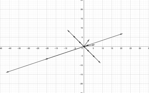
::让我们尝试几个数字的例子 然后我们展示一些惊人的几何解释 与一些有用的身份和定理

First, let's keep it simple and try out a 2x2 matrix. Let  $\begin{align*}A=\begin{bmatrix}6 & 3\\-1 & 4\end{bmatrix}\end{align*}$ . Now  $\begin{align*}A-\lambda\cdot I = \begin{bmatrix}6-\lambda & 3\\1 & 4-\lambda\end{bmatrix}\end{align*}$  so now  $\begin{align*}\text{det}(A-\lambda\cdot I) = (6-\lambda)\cdot(4-\lambda) - 3 = 24 + \lambda^{2} - 10\cdot\lambda - 3 = \lambda^{2} - 10\cdot\lambda + 21 = (\lambda - 7)\cdot(\lambda - 3)\end{align*}$  and from here we get that our eigenvalues are  $\begin{align*}\lambda = 3 \text{ and } \lambda = 7\end{align*}$ . Now we know that  $\begin{align*}T(\vec{x})\end{align*}$  is a scalar multiple of the input vector if and only if  $\begin{align*}T(\vec{x}) = 7\cdot\vec{x} \text{ or } 3\cdot\vec{x}\end{align*}$  and in later lessons we will learn some algebraic techniques of how to find these vectors  $\begin{align*}\vec{x}\end{align*}$  where this is true.
::首先,让我们保持简单并尝试 2x2 矩阵。 让我们 A = [63- 14] 。 现在 AI = [6314] 。 现在, AI = [6314] 。 现在, 现在, I = (6) (4) - (4) - 3= 242 - 1032 - 1021 = (7) 3⁄2 - 10 21 = (7) 3⁄7 。 现在我们知道, T (x) 是输入矢量的一个斜体, 只有当 T( x) = 7x 或 3x 并在以后的教学中学习一些代数技术, 如何找到这些矢量 x 。

We can now analyze how this happens geometrically and look at those eigenvalues in the transformation.
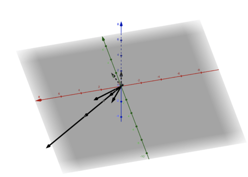
::我们现在可以从几何角度分析 如何发生这种变化 并观察这些变异中的自然价值