用Python运行一个神经网络(Running a Neural Network with Python)
章节大纲
-
神经网络类
 在我们的神经网络教程上一章中,我们学习了关于权重最重要的事实。我们了解了它们是如何使用的以及如何在 Python 中实现它们。我们看到,权值与输入值的乘法可以通过应用矩阵乘法来使用 NumPy 数组完成。
然而,我们还没有在一个真实的神经网络环境中测试它们。我们必须首先创建这个环境。我们现在将在 Python 中创建一个实现神经网络的类。我们将循序渐进,以便一切都易于理解。
我们的类最基本的方法是:
-
__init__: 用于初始化一个类,即我们将设置每一层的神经元数量并初始化权重矩阵。 -
run: 应用于我们要分类的样本的方法。它将此样本应用于神经网络。我们可以说,我们“运行”网络来“预测”结果。这个方法在其他实现中通常被称为predict。 -
train: 这个方法将样本和相应的目标值作为输入。有了这些输入,它可以在必要时调整权重值。这意味着网络从输入中学习。从用户的角度来看,我们“训练”网络。例如,在 scikit-learn 中,这个方法被称为fit。
我们将把
train和run方法的定义推迟到后面。权重矩阵应该在__init__方法内部初始化。我们间接地这样做。我们定义一个方法create_weight_matrices并在__init__中调用它。这样,init方法保持清晰。我们还将推迟向层中添加偏置节点。
下面的 Python 代码包含了一个神经网络类的实现,应用了我们在上一章中学习到的知识:
Pythonimport numpy as np from scipy.stats import truncnorm def truncated_normal(mean=0, sd=1, low=0, upp=10): return truncnorm( (low - mean) / sd, (upp - mean) / sd, loc=mean, scale=sd) class NeuralNetwork: def __init__(self, no_of_in_nodes, no_of_out_nodes, no_of_hidden_nodes, learning_rate): self.no_of_in_nodes = no_of_in_nodes self.no_of_out_nodes = no_of_out_nodes self.no_of_hidden_nodes = no_of_hidden_nodes self.learning_rate = learning_rate self.create_weight_matrices() def create_weight_matrices(self): """ A method to initialize the weight matrices of the neural network""" rad = 1 / np.sqrt(self.no_of_in_nodes) X = truncated_normal(mean=0, sd=1, low=-rad, upp=rad) self.weights_in_hidden = X.rvs((self.no_of_hidden_nodes, self.no_of_in_nodes)) rad = 1 / np.sqrt(self.no_of_hidden_nodes) X = truncated_normal(mean=0, sd=1, low=-rad, upp=rad) self.weights_hidden_out = X.rvs((self.no_of_out_nodes, self.no_of_hidden_nodes)) def train(self): pass def run(self): pass我们无法用这段代码做很多事情,但我们至少可以初始化它。我们还可以看看权重矩阵:
Pythonsimple_network = NeuralNetwork(no_of_in_nodes = 3, no_of_out_nodes = 2, no_of_hidden_nodes = 4, learning_rate = 0.1) print(simple_network.weights_in_hidden) print(simple_network.weights_hidden_out)输出:
[[-0.3460287  -0.19427278 -0.19102916]
 [ 0.56743476 -0.47164202 -0.06910573]
 [ 0.53013469 -0.05117752 -0.430623  ]
 [ 0.48414483  0.31263278 -0.08123676]]
[[-0.12645547  0.05260599 -0.36278102 -0.32649173]
 [-0.20841352 -0.01456191 -0.13778649 -0.08920465]]
激活函数、Sigmoid 和 ReLU
在我们可以编写
run方法之前,我们必须处理激活函数。在神经网络的介绍章节中,我们有以下图示: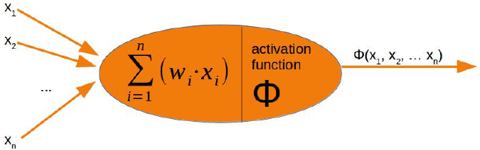
感知器的输入值由求和函数处理,然后由激活函数转换,将求和函数的输出转换为所需且更合适的输出。求和函数意味着我们将对权重向量和输入值进行矩阵乘法。
神经网络中使用了许多不同的激活函数。关于可能的激活函数最全面的概述之一可以在维基百科上找到。
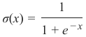
Sigmoid 函数是常用激活函数之一。我们正在使用的 Sigmoid 函数也称为逻辑函数。
它被定义为:
让我们看看 Sigmoid 函数的图。我们使用 Matplotlib 绘制 Sigmoid 函数:
Pythonimport numpy as np import matplotlib.pyplot as plt def sigma(x): return 1 / (1 + np.exp(-x)) X = np.linspace(-5, 5, 100) plt.plot(X, sigma(X),'b') plt.xlabel('X Axis') plt.ylabel('Y Axis') plt.title('Sigmoid Function') plt.grid() plt.text(2.3, 0.84, r'$\sigma(x)=\frac{1}{1+e^{-x}}$', fontsize=16) plt.show()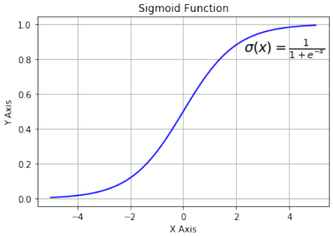
观察图表,我们可以看到 Sigmoid 函数将给定的数字 x 映射到 0 到 1 之间的数字范围。不包括 0 和 1!随着 x 值变大,Sigmoid 函数的值越来越接近 1;随着 x 值变小,Sigmoid 函数的值越来越接近 0。
除了我们自己定义 Sigmoid 函数外,我们还可以使用
scipy.special中的expit函数,它是 Sigmoid 函数的一种实现。它可以应用于各种数据类型,如int、float、list、numpy.ndarray等。结果是一个与输入数据 x 形状相同的ndarray。Pythonfrom scipy.special import expit print(expit(3.4)) print(expit([3, 4, 1])) print(expit(np.array([0.8, 2.3, 8])))输出:
0.9677045353015494 [0.95257413 0.98201379 0.73105858] [0.68997448 0.90887704 0.99966465]逻辑函数在神经网络中经常用于引入非线性并将信号映射到指定范围,即 0 和 1。它也广受欢迎,因为其导数(在反向传播中需要)很简单。
及其导数:
 Python
import numpy as np import matplotlib.pyplot as plt def sigma(x): return 1 / (1 + np.exp(-x)) X = np.linspace(-5, 5, 100) plt.plot(X, sigma(X)) plt.plot(X, sigma(X) * (1 - sigma(X))) plt.xlabel('X Axis') plt.ylabel('Y Axis') plt.title('Sigmoid Function') plt.grid() plt.text(2.3, 0.84, r'$\sigma(x)=\frac{1}{1+e^{-x}}$', fontsize=16) plt.text(0.3, 0.1, r'$\sigma\'(x) = \sigma(x)(1 - \sigma(x))$', fontsize=16) plt.show()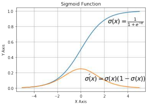
我们也可以用 NumPy 的装饰器
vectorize定义我们自己的 Sigmoid 函数:Python@np.vectorize def sigmoid(x): return 1 / (1 + np.e ** -x) #sigmoid = np.vectorize(sigmoid) sigmoid([3, 4, 5])输出:
array([0.95257413, 0.98201379, 0.99330715])另一个易于使用的激活函数是 ReLU 函数。ReLU 代表修正线性单元。它也称为斜坡函数。它被定义为其参数的正部分,即 。这“目前是最成功和广泛使用的激活函数是修正线性单元(ReLU)”[^1]。ReLU 函数比 Sigmoid 类函数在计算上更高效,因为 ReLU 只需在 0 和参数 x 之间选择最大值。而 Sigmoid 函数需要执行昂贵的指数运算。
Python# alternative activation function def ReLU(x): return np.maximum(0.0, x) # derivation of relu def ReLU_derivation(x): if x <= 0: return 0 else: return 1Pythonimport numpy as np import matplotlib.pyplot as plt X = np.linspace(-5, 6, 100) plt.plot(X, ReLU(X),'b') plt.xlabel('X Axis') plt.ylabel('Y Axis') plt.title('ReLU Function') plt.grid() plt.text(0.8, 0.4, r'$ReLU(x)=max(0, x)$', fontsize=14) plt.show()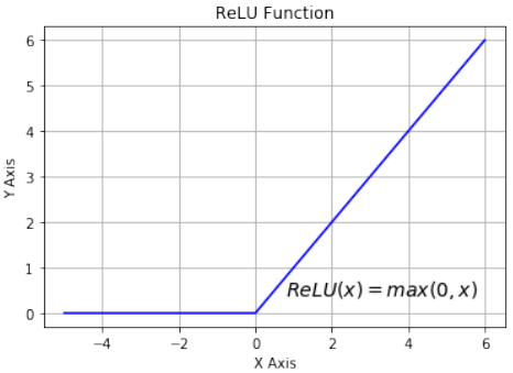
添加
run方法我们现在已经准备好实现神经网络类的
run(或predict)方法。我们将使用scipy.special作为激活函数并将其重命名为activation_function:Pythonfrom scipy.special import expit as activation_functionrun方法中我们要做的所有事情包括以下几点:-
输入向量与
weights_in_hidden矩阵的矩阵乘法。 -
对步骤 1 的结果应用激活函数。
-
步骤 2 的结果向量与
weights_hidden_out矩阵的矩阵乘法。 -
为了得到最终结果:对步骤 3 的结果应用激活函数。
Pythonimport numpy as np from scipy.special import expit as activation_function from scipy.stats import truncnorm def truncated_normal(mean=0, sd=1, low=0, upp=10): return truncnorm( (low - mean) / sd, (upp - mean) / sd, loc=mean, scale=sd) class NeuralNetwork: def __init__(self, no_of_in_nodes, no_of_out_nodes, no_of_hidden_nodes, learning_rate): self.no_of_in_nodes = no_of_in_nodes self.no_of_out_nodes = no_of_out_nodes self.no_of_hidden_nodes = no_of_hidden_nodes self.learning_rate = learning_rate self.create_weight_matrices() def create_weight_matrices(self): """ 一个用于初始化神经网络权重矩阵的方法 """ rad = 1 / np.sqrt(self.no_of_in_nodes) X = truncated_normal(mean=0, sd=1, low=-rad, upp=rad) self.weights_in_hidden = X.rvs((self.no_of_hidden_nodes, self.no_of_in_nodes)) rad = 1 / np.sqrt(self.no_of_hidden_nodes) X = truncated_normal(mean=0, sd=1, low=-rad, upp=rad) self.weights_hidden_out = X.rvs((self.no_of_out_nodes, self.no_of_hidden_nodes)) def train(self, input_vector, target_vector): pass def run(self, input_vector): """ 使用输入向量 'input_vector' 运行网络。 'input_vector' 可以是元组、列表或 ndarray。 """ # 将输入向量转换为列向量 input_vector = np.array(input_vector, ndmin=2).T # 计算隐藏层输入并应用激活函数 input_hidden = activation_function(self.weights_in_hidden @ input_vector) # 计算输出层输入并应用激活函数 output_vector = activation_function(self.weights_hidden_out @ input_hidden) return output_vector我们可以实例化这个类,它将是一个神经网络。在下面的示例中,我们创建一个具有两个输入节点、四个隐藏节点和两个输出节点的网络。
Pythonsimple_network = NeuralNetwork(no_of_in_nodes=2, no_of_out_nodes=2, no_of_hidden_nodes=4, learning_rate=0.6)我们可以将
run方法应用于所有形状为(2,)的数组,以及包含两个数字元素的列表和元组。函数调用的结果由权重的随机值决定:Pythonsimple_network.run([(3, 4)])输出:
array([[0.54558831], [0.6834667 ]])
注脚
[^1]:
Ramachandran, Prajit; Barret, Zoph; Quoc, V. Le (October 16, 2017). "Searching for Activation Functions".
A NEURAL NETWORK CLASS
We learned in the previous chapter of our tutorial on neural
networks the most important facts about weights. We saw how
they are used and how we can implement them in Python. We
saw that the multiplication of the weights with the input values
can be accomplished with arrays from Numpy by applying
matrix multiplication.
However, what we hadn't done was to test them in a real neural
network environment. We have to create this environment first.
We will now create a class in Python, implementing a neural
network. We will proceed in small steps so that everything is
easy to understand.
The most essential methods our class needs are:
•••__init__ to initialize a class, i.e. we will set
the number of neurons for every layer and
initialize the weight matrices.
run : A method which is applied to a sample,
which which we want to classify. It applies this
sample to the neural network. We could say, we
'run' the network to 'predict' the result. This
method is in other implementations often known
as predict .
train : This method gets a sample and the corresponding target value as an input. With this
input it can adjust the weight values if necessary. This means the network learns from an input.
Seen from the user point of view, we 'train' the network. In sklearn for example, this method
is called fit
We will postpone the definition of the train and run method until later. The weight matrices should be
initialized inside of the __init__ method. We do this indirectly. We define a method
create_weight_matrices and call it in __init__ . In this way, the init method remains clear.
We will also postpone adding bias nodes to the layers.
153
The following Python code contains an implementation of a neural network class applying the knowledge we
worked out in the previous chapter:
import numpy as np
from scipy.stats import truncnorm
def truncated_normal(mean=0, sd=1, low=0, upp=10):
return truncnorm(
(low - mean) / sd, (upp - mean) / sd, loc=mean, scale=sd)
class NeuralNetwork:
def __init__(self,
no_of_in_nodes,
no_of_out_nodes,
no_of_hidden_nodes,
learning_rate):
self.no_of_in_nodes = no_of_in_nodes
self.no_of_out_nodes = no_of_out_nodes
self.no_of_hidden_nodes = no_of_hidden_nodes
self.learning_rate = learning_rate
self.create_weight_matrices()
def create_weight_matrices(self):
rad = 1 / np.sqrt(self.no_of_in_nodes)
X = truncated_normal(mean=0, sd=1, low=-rad, upp=rad)
self.weights_in_hidden = X.rvs((self.no_of_hidden_nodes,
self.no_of_in_nodes))
rad = 1 / np.sqrt(self.no_of_hidden_nodes)
X = truncated_normal(mean=0, sd=1, low=-rad, upp=rad)
self.weights_hidden_out = X.rvs((self.no_of_out_nodes,
self.no_of_hidden_nodes))
deftrain(self):
pass
defrun(self):
pass
We cannot do a lot with this code, but we can at least initialize it. We can also have a look at the weight
matrices:
simple_network = NeuralNetwork(no_of_in_nodes = 3,
154
no_of_out_nodes = 2,
no_of_hidden_nodes = 4,
learning_rate = 0.1)
print(simple_network.weights_in_hidden)
print(simple_network.weights_hidden_out)
[[-0.3460287 -0.19427278 -0.19102916]
[ 0.56743476 -0.47164202 -0.06910573]
[ 0.53013469 -0.05117752 -0.430623 ]
[ 0.48414483 0.31263278 -0.08123676]]
[[-0.12645547 0.05260599 -0.36278102 -0.32649173]
[-0.20841352 -0.01456191 -0.13778649 -0.08920465]]
ACTIVATION FUNCTIONS, SIGMOID AND RELU
Before we can program the run method, we have to deal with the activation function. We had the following
diagram in the introductory chapter on neural networks:
The input values of a perceptron are processed by the summation function and followed by an activation
function, transforming the output of the summation function into a desired and more suitable output. The
summation function means that we will have a matrix multiplication of the weight vectors and the input
values.
There are lots of different activation functions used in neural networks. One of the most comprehensive
overviews of possible activation functions can be found at Wikipedia.
The sigmoid function is one of the often used activation functions. The sigmoid function, which we are using,
is also known as the Logistic function.
It is defined as
1
σ(x) =
1 + e − x
Let us have a look at the graph of the sigmoid function. We use matplotlib to plot the sigmoid function:
import numpy as np
155
import matplotlib.pyplot as plt
def sigma(x):
return 1 / (1 + np.exp(-x))
X = np.linspace(-5, 5, 100)
plt.plot(X, sigma(X),'b')
plt.xlabel('X Axis')
plt.ylabel('Y Axis')
plt.title('Sigmoid Function')
plt.grid()
plt.text(2.3, 0.84, r'$\sigma(x)=\frac{1}{1+e^{-x}}$', fontsize=1
6)
plt.show()
Looking at the graph, we can see that the sigmoid function maps a given number x into the range of numbers
between 0 and 1. 0 and 1 not included! As the value of x gets larger, the value of the sigmoid function gets
closer and closer to 1 and as x gets smaller, the value of the sigmoid function is approaching 0.
Instead of defining the sigmoid function ourselves, we can also use the expit function from
scipy.special , which is an implementation of the sigmoid function. It can be applied on various data
classes like int, float, list, numpy,ndarray and so on. The result is an ndarray of the same shape as the input
data x.
156
from scipy.special import expit

print(expit(3.4))
print(expit([3, 4, 1]))
print(expit(np.array([0.8, 2.3, 8])))
0.9677045353015494
[0.95257413 0.98201379 0.73105858]
[0.68997448 0.90887704 0.99966465]
The logistic function is often often used in neural networks to introduce nonlinearity in the model and to map
signals into a specified range, i.e. 0 and 1. It is also well liked because the derivative - needed in
backpropagation - is simple.
1
σ(x) =
1 + e − x
and its derivative:
σ ′ (x) = σ(x)(1 − σ(x))
import numpy as np
import matplotlib.pyplot as plt
def sigma(x):
return 1 / (1 + np.exp(-x))
X = np.linspace(-5, 5, 100)
plt.plot(X, sigma(X))
plt.plot(X, sigma(X) * (1 - sigma(X)))
plt.xlabel('X Axis')
plt.ylabel('Y Axis')
plt.title('Sigmoid Function')
plt.grid()
plt.text(2.3, 0.84, r'$\sigma(x)=\frac{1}{1+e^{-x}}$', fontsize=1
6)
plt.text(0.3, 0.1, r'$\sigma\'(x) = \sigma(x)(1 - \sigma(x))$', fo
ntsize=16)
plt.show()
157
We can also define our own sigmoid function with the decorator vectorize from numpy:
@np.vectorize
def sigmoid(x):
    return 1 / (1 + np.e ** -x)

#sigmoid = np.vectorize(sigmoid)
sigmoid([3, 4, 5])
Output:array([0.95257413, 0.98201379, 0.99330715])
Another easy to use activation function is the ReLU function. ReLU stands for rectified linear unit. It is also
known as the ramp function. It is defined as the positve part of its argument, i.e. y = max (0, x). This is
"currently, the most successful and widely-used activation function is the Rectified Linear Unit (ReLU)" 1 The
ReLu function is computationally more efficient than Sigmoid like functions, because Relu means only
choosing the maximum between 0 and the argument x . Whereas Sigmoids need to perform expensive
exponential operations.
# alternative activation function
def ReLU(x):
    return np.maximum(0.0, x)

# derivation of relu
def ReLU_derivation(x):
    if x <= 0:
        return 0
    else:
        return 1
158
import numpy as np
import matplotlib.pyplot as plt

X = np.linspace(-5, 6, 100)
plt.plot(X, ReLU(X),'b')
plt.xlabel('X Axis')
plt.ylabel('Y Axis')
plt.title('ReLU Function')
plt.grid()
plt.text(0.8, 0.4, r'$ReLU(x)=max(0, x)$', fontsize=14)
plt.show()
ADDING A RUN METHOD
We have everything together now to implement the run (or predict ) method of our neural network
class. We will use scipy.special as the activation function and rename it to
activation_function :
from scipy.special import expit as activation_function
All we have to do in the run method consists of the following.
1.
2.
3.
4.
Matrix multiplication of the input vector and the weights_in_hidden matrix.
Applying the activation function to the result of step 1
Matrix multiplication of the result vector of step 2 and the weights_in_hidden matrix.
To get the final result: Applying the activation function to the result of 3
import numpy as np
from scipy.special import expit as activation_function
159
from scipy.stats import truncnorm
def truncated_normal(mean=0, sd=1, low=0, upp=10):
return truncnorm(
(low - mean) / sd, (upp - mean) / sd, loc=mean, scale=sd)
class NeuralNetwork:
def __init__(self,
no_of_in_nodes,
no_of_out_nodes,
no_of_hidden_nodes,
learning_rate):
self.no_of_in_nodes = no_of_in_nodes
self.no_of_out_nodes = no_of_out_nodes
self.no_of_hidden_nodes = no_of_hidden_nodes
self.learning_rate = learning_rate
self.create_weight_matrices()
def create_weight_matrices(self):
""" A method to initialize the weight matrices of the neur
al network"""
rad = 1 / np.sqrt(self.no_of_in_nodes)
X = truncated_normal(mean=0, sd=1, low=-rad, upp=rad)
self.weights_in_hidden = X.rvs((self.no_of_hidden_nodes,
self.no_of_in_nodes))
rad = 1 / np.sqrt(self.no_of_hidden_nodes)
X = truncated_normal(mean=0, sd=1, low=-rad, upp=rad)
self.weights_hidden_out = X.rvs((self.no_of_out_nodes,
self.no_of_hidden_nodes))
def train(self, input_vector, target_vector):
pass
def run(self, input_vector):
"""
running the network with an input vector 'input_vector'.
'input_vector' can be tuple, list or ndarray
"""
# turning the input vector into a column vector
input_vector = np.array(input_vector, ndmin=2).T
input_hidden = activation_function(self.weights_in_hidden
160
@ input_vector)
output_vector = activation_function(self.weights_hidden_ou
t @ input_hidden)
return output_vector
We can instantiate an instance of this class, which will be a neural network. In the following example we
create a network with two input nodes, four hidden nodes, and two output nodes.
simple_network = NeuralNetwork(no_of_in_nodes=2,
                               no_of_out_nodes=2,
                               no_of_hidden_nodes=4,
                               learning_rate=0.6)
We can apply the run method to all arrays with a shape of (2,), also lists and tuples with two numerical
elements. The result of the call is defined by the random values of the weights:
simple_network.run([(3, 4)])
Output:array([[0.54558831],
[0.6834667 ]])
FOOTNOTES
1
Ramachandran, Prajit; Barret, Zoph; Quoc, V. Le (October 16, 2017). "Searching for Activation Functions". -