节: 神经网络（Neural Network） | 机器学习Python教程

章节大纲

使用 MNIST

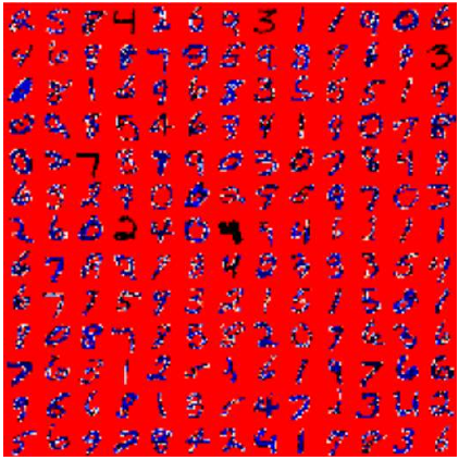
MNIST 数据库（修改后的美国国家标准与技术研究院数据库）的手写数字包含一个 60,000 个示例的训练集和一个 10,000 个示例的测试集。它是 NIST 提供的更大数据集的子集。此外，NIST 的黑白图像经过大小归一化和居中处理，以适应 28x28 像素的包围盒并进行抗锯齿处理，这引入了灰度级别。

这个数据库因其在机器学习和图像处理领域的训练和测试而备受青睐。它是原始 NIST 数据集的重混子集。60,000 张训练图像中的一半来自 NIST 的测试数据集，另一半来自 NIST 的训练集。10,000 张测试集图像也以类似方式组装。

MNIST 数据集被研究人员用于测试和比较他们的研究结果。文献中最低的错误率低至 0.21%。

读取 MNIST 数据集

数据集中的图像大小为 28 x 28 像素。它们保存在 CSV 数据文件 mnist_train.csv 和 mnist_test.csv 中。

这些文件中的每一行都包含一个图像，即 785 个介于 0 到 255 之间的数字。

每行的第一个数字是标签，即图像中描绘的数字。接下来的 784 个数字是 28 x 28 图像的像素值。

Python

import numpy as np
import matplotlib.pyplot as plt

image_size = 28 # 宽度和长度
no_of_different_labels = 10 # 即 0, 1, 2, ..., 9
image_pixels = image_size * image_size # 28 * 28 = 784 像素
data_path = "data/mnist/" # 确保 'data/mnist/' 路径下有 csv 文件

# 加载训练数据和测试数据
train_data = np.loadtxt(data_path + "mnist_train.csv",
                        delimiter=",")
test_data = np.loadtxt(data_path + "mnist_test.csv",
                       delimiter=",")

# 查看测试数据的前10行
print("测试数据前10行:")
print(test_data[:10])

# 检查数据中值为255的元素（可选）
# print("值为255的元素数量:", test_data[test_data==255].size)

# 检查测试数据的形状
print("测试数据形状:", test_data.shape)

输出：

测试数据前10行:
[[7. 0. 0. ... 0. 0. 0.]
 [2. 0. 0. ... 0. 0. 0.]
 [1. 0. 0. ... 0. 0. 0.]
 ...
 [9. 0. 0. ... 0. 0. 0.]
 [5. 0. 0. ... 0. 0. 0.]
 [9. 0. 0. ... 0. 0. 0.]]
测试数据形状: (10000, 785)

MNIST 数据集的图像是灰度图像，像素值介于 0 到 255 之间（包括两端值）。我们将通过将每个像素乘以 0.99 / 255 并加上 0.01 来将这些值映射到 [0.01, 1] 的区间。这样，我们避免了输入值为 0 的情况，正如我们在介绍章节中看到的那样，0 值会阻止权重更新。

Python

fac = 0.99 / 255
# 提取图像数据（除了第一列的标签），并进行缩放和偏移
train_imgs = np.asfarray(train_data[:, 1:]) * fac + 0.01
test_imgs = np.asfarray(test_data[:, 1:]) * fac + 0.01

# 提取标签数据（第一列）
train_labels = np.asfarray(train_data[:, :1])
test_labels = np.asfarray(test_data[:, :1])

在我们的计算中，我们需要独热 (one-hot) 表示的标签。我们有 0 到 9 的 10 个数字，即 lr = np.arange(10)。

将标签转换为独热表示可以通过命令 (lr==label).astype(np.int) 实现。

我们通过以下示例演示：

Python

import numpy as np

lr = np.arange(10)
for label in range(10):
    one_hot = (lr==label).astype(np.int) # 使用 np.int 或 np.int32/np.int64
    print("label: ", label, " in one-hot representation: ", one_hot)

输出：

label:  0  in one-hot representation:  [1 0 0 0 0 0 0 0 0 0]
label:  1  in one-hot representation:  [0 1 0 0 0 0 0 0 0 0]
label:  2  in one-hot representation:  [0 0 1 0 0 0 0 0 0 0]
label:  3  in one-hot representation:  [0 0 0 1 0 0 0 0 0 0]
label:  4  in one-hot representation:  [0 0 0 0 1 0 0 0 0 0]
label:  5  in one-hot representation:  [0 0 0 0 0 1 0 0 0 0]
label:  6  in one-hot representation:  [0 0 0 0 0 0 1 0 0 0]
label:  7  in one-hot representation:  [0 0 0 0 0 0 0 1 0 0]
label:  8  in one-hot representation:  [0 0 0 0 0 0 0 0 1 0]
label:  9  in one-hot representation:  [0 0 0 0 0 0 0 0 0 1]

现在我们准备将带标签的图像转换为独热表示。我们创建 0.01 和 0.99 而不是 0 和 1，这对于我们的计算会更好：

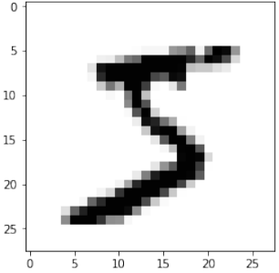
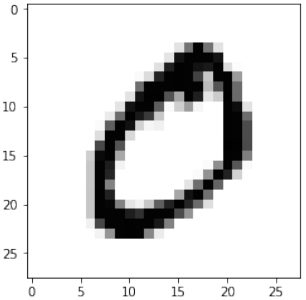
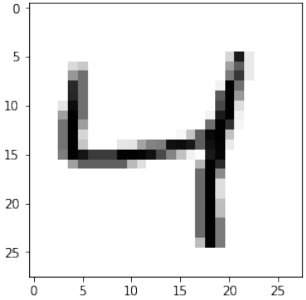
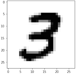
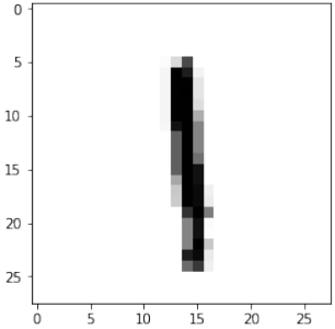
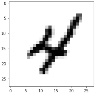
Python

lr = np.arange(no_of_different_labels)

# 将标签转换为独热表示
train_labels_one_hot = (lr==train_labels).astype(np.float64) # 使用 np.float64
test_labels_one_hot = (lr==test_labels).astype(np.float64)   # 使用 np.float64

# 将独热标签中的 0 变为 0.01，1 变为 0.99
train_labels_one_hot[train_labels_one_hot==0] = 0.01
train_labels_one_hot[train_labels_one_hot==1] = 0.99
test_labels_one_hot[test_labels_one_hot==0] = 0.01
test_labels_one_hot[test_labels_one_hot==1] = 0.99

在我们开始将 MNIST 数据集用于神经网络之前，我们先看看一些图像：

Python

for i in range(10):
    img = train_imgs[i].reshape((28,28))
    plt.imshow(img, cmap="Greys")
    plt.title(f"Label: {int(train_labels[i][0])}") # 显示图像对应的标签
    plt.show()

快速重新加载的数据转储

您可能已经注意到从 CSV 文件读取数据相当慢。

我们将使用 pickle 模块的 dump 函数以二进制格式保存数据：

Python

import pickle

# 确保 'data/mnist/' 目录存在
import os
os.makedirs("data/mnist/", exist_ok=True)

with open("data/mnist/pickled_mnist.pkl", "bw") as fh:
    data = (train_imgs,
            test_imgs,
            train_labels,
            test_labels,
            train_labels_one_hot,
            test_labels_one_hot)
    pickle.dump(data, fh)

现在我们可以使用 pickle.load 读取数据了。这比使用 loadtxt 读取 CSV 文件快得多：

Python

import pickle

with open("data/mnist/pickled_mnist.pkl", "br") as fh:
    data = pickle.load(fh)

train_imgs = data[0]
test_imgs = data[1]
train_labels = data[2]
test_labels = data[3]
train_labels_one_hot = data[4]
test_labels_one_hot = data[5]

image_size = 28 # 宽度和长度
no_of_different_labels = 10 # 即 0, 1, 2, ..., 9
image_pixels = image_size * image_size

数据分类

我们将使用以下神经网络类进行我们的首次分类：

Python

import numpy as np

@np.vectorize
def sigmoid(x):
    return 1 / (1 + np.e ** -x)

activation_function = sigmoid

from scipy.stats import truncnorm

def truncated_normal(mean=0, sd=1, low=0, upp=10):
    return truncnorm((low - mean) / sd,
                     (upp - mean) / sd,
                     loc=mean,
                     scale=sd)

class NeuralNetwork:
    def __init__(self,
                 no_of_in_nodes,
                 no_of_out_nodes,
                 no_of_hidden_nodes,
                 learning_rate):
        self.no_of_in_nodes = no_of_in_nodes
        self.no_of_out_nodes = no_of_out_nodes
        self.no_of_hidden_nodes = no_of_hidden_nodes
        self.learning_rate = learning_rate
        self.create_weight_matrices()

    def create_weight_matrices(self):
        """
        一个初始化神经网络权重矩阵的方法
        """
        rad = 1 / np.sqrt(self.no_of_in_nodes)
        X = truncated_normal(mean=0,
                             sd=1,
                             low=-rad,
                             upp=rad)
        self.wih = X.rvs((self.no_of_hidden_nodes,
                          self.no_of_in_nodes)) # 输入层到隐藏层权重

        rad = 1 / np.sqrt(self.no_of_hidden_nodes)
        X = truncated_normal(mean=0, sd=1, low=-rad, upp=rad)
        self.who = X.rvs((self.no_of_out_nodes,
                          self.no_of_hidden_nodes)) # 隐藏层到输出层权重

    def train(self, input_vector, target_vector):
        """
        input_vector 和 target_vector 可以是元组、列表或 ndarray
        """
        # 将输入和目标向量转换为列向量
        input_vector = np.array(input_vector, ndmin=2).T
        target_vector = np.array(target_vector, ndmin=2).T

        # 前向传播
        output_vector1 = np.dot(self.wih, input_vector)
        output_hidden = activation_function(output_vector1)

        output_vector2 = np.dot(self.who, output_hidden)
        output_network = activation_function(output_vector2)

        # 计算误差
        output_errors = target_vector - output_network

        # 更新隐藏层到输出层的权重 (who)
        tmp = output_errors * output_network * (1.0 - output_network)
        tmp = self.learning_rate * np.dot(tmp, output_hidden.T)
        self.who += tmp

        # 计算隐藏层误差
        hidden_errors = np.dot(self.who.T, output_errors)

        # 更新输入层到隐藏层的权重 (wih)
        tmp = hidden_errors * output_hidden * (1.0 - output_hidden)
        self.wih += self.learning_rate * np.dot(tmp, input_vector.T)

    def run(self, input_vector):
        # input_vector 可以是元组、列表或 ndarray
        input_vector = np.array(input_vector, ndmin=2).T
        
        # 前向传播
        output_vector = np.dot(self.wih, input_vector)
        output_vector = activation_function(output_vector)
        output_vector = np.dot(self.who, output_vector)
        output_vector = activation_function(output_vector)
        return output_vector

    def confusion_matrix(self, data_array, labels):
        cm = np.zeros((10, 10), int) # 10x10 的混淆矩阵
        for i in range(len(data_array)):
            res = self.run(data_array[i])
            res_max = res.argmax() # 预测的类别（索引）
            target = int(labels[i][0]) # 真实的类别（从 [标签.] 中提取整数）
            cm[res_max, target] += 1 # 预测为 res_max，实际为 target
        return cm

    def precision(self, label, confusion_matrix):
        col = confusion_matrix[:, label] # 预测为该标签的所有样本（列）
        return confusion_matrix[label, label] / col.sum()

    def recall(self, label, confusion_matrix):
        row = confusion_matrix[label, :] # 实际为该标签的所有样本（行）
        return confusion_matrix[label, label] / row.sum()

    def evaluate(self, data, labels):
        corrects, wrongs = 0, 0
        for i in range(len(data)):
            res = self.run(data[i])
            res_max = res.argmax() # 预测的类别
            if res_max == int(labels[i][0]): # 比较预测类别和实际类别（提取整数值）
                corrects += 1
            else:
                wrongs += 1
        return corrects, wrongs

# --- 实例化并训练神经网络 ---
ANN = NeuralNetwork(no_of_in_nodes = image_pixels,
                    no_of_out_nodes = 10,
                    no_of_hidden_nodes = 100, # 隐藏层节点数
                    learning_rate = 0.1)     # 学习率

# 训练网络
print("开始训练网络...")
epochs = 5 # 增加训练轮次，可以进一步提高准确率
for epoch in range(epochs):
    print(f"Epoch {epoch+1}/{epochs}")
    for i in range(len(train_imgs)):
        ANN.train(train_imgs[i], train_labels_one_hot[i])
print("训练完成。")

# 对测试集前20个样本进行预测并打印结果
print("\n测试集前20个样本的预测结果:")
for i in range(20):
    res = ANN.run(test_imgs[i])
    print(f"真实标签: {int(test_labels[i][0])}, 预测标签: {np.argmax(res)}, 最大预测概率: {np.max(res):.4f}")

# 评估训练集和测试集的准确率
corrects_train, wrongs_train = ANN.evaluate(train_imgs, train_labels)
print("\n训练集准确率: ", corrects_train / ( corrects_train + wrongs_train))

corrects_test, wrongs_test = ANN.evaluate(test_imgs, test_labels)
print("测试集准确率: ", corrects_test / ( corrects_test + wrongs_test))

# 计算混淆矩阵
cm = ANN.confusion_matrix(train_imgs, train_labels) # 可以计算训练集或测试集的混淆矩阵
print("\n训练集混淆矩阵:")
print(cm)

# 计算并打印每个数字的精确率和召回率
print("\n每个数字的精确率和召回率:")
for i in range(10):
    # 确保分母不为零，避免除以零的警告
    prec = ANN.precision(i, cm) if cm[:, i].sum() > 0 else np.nan
    rec = ANN.recall(i, cm) if cm[i, :].sum() > 0 else np.nan
    print(f"数字: {i}, 精确率: {prec:.4f}, 召回率: {rec:.4f}")

输出示例（由于随机初始化和训练过程，具体数字可能会略有不同）：

开始训练网络...
Epoch 1/5
...
Epoch 5/5
训练完成。

测试集前20个样本的预测结果:
真实标签: 7, 预测标签: 7, 最大预测概率: 0.9829
真实标签: 2, 预测标签: 2, 最大预测概率: 0.7373
真实标签: 1, 预测标签: 1, 最大预测概率: 0.9882
真实标签: 0, 预测标签: 0, 最大预测概率: 0.9873
真实标签: 4, 预测标签: 4, 最大预测概率: 0.9456
真实标签: 1, 预测标签: 1, 最大预测概率: 0.9880
真实标签: 4, 预测标签: 4, 最大预测概率: 0.9766
真实标签: 9, 预测标签: 9, 最大预测概率: 0.9649
真实标签: 5, 预测标签: 6, 最大预测概率: 0.3662  <-- 这是一个错误分类示例
真实标签: 9, 预测标签: 9, 最大预测概率: 0.9849
真实标签: 0, 预测标签: 0, 最大预测概率: 0.9204
真实标签: 6, 预测标签: 6, 最大预测概率: 0.8898
真实标签: 9, 预测标签: 9, 最大预测概率: 0.9937
真实标签: 0, 预测标签: 0, 最大预测概率: 0.9832
真实标签: 1, 预测标签: 1, 最大预测概率: 0.9888
真实标签: 5, 预测标签: 5, 最大预测概率: 0.9157
真实标签: 9, 预测标签: 9, 最大预测概率: 0.9813
真实标签: 7, 预测标签: 7, 最大预测概率: 0.9889
真实标签: 3, 预测标签: 3, 最大预测概率: 0.8773
真实标签: 4, 预测标签: 4, 最大预测概率: 0.9900

训练集准确率:  0.9469166666666666
测试集准确率:  0.9459

训练集混淆矩阵:
[[5802    1    5    6    8    5   37    0   52    7]
 [   0 6620   22   36   16    2    4    5   20   17]
 [  53   45 5486  114   54    3   54   31  103   15]
 [  21   22   51 5788    8   44   19   38   83   57]
 [   9    6   10    2 5439    0   71    7    9  289]
 [  42   29   11  114   41 4922   72    4  102   84]
 [  35   14    5    1   10   20 5789    0   43    1]
 [   8   50   53   35   52    3    3 5762   21  278]
 [  14   75   11   76   25    5   41    1 5535   68]
 [  20    7    3   72   90   11    4   32   38 5672]]

每个数字的精确率和召回率:
数字: 0, 精确率: 0.9796, 召回率: 0.9664
数字: 1, 精确率: 0.9819, 召回率: 0.9638
数字: 2, 精确率: 0.9208, 召回率: 0.9698
数字: 3, 精确率: 0.9441, 召回率: 0.9270
数字: 4, 精确率: 0.9310, 召回率: 0.9471
数字: 5, 精确率: 0.9080, 召回率: 0.9815
数字: 6, 精确率: 0.9782, 召回率: 0.9499
数字: 7, 精确率: 0.9197, 召回率: 0.9799
数字: 8, 精确率: 0.9460, 召回率: 0.9216
数字: 9, 精确率: 0.9534, 召回率: 0.8742

USING MNIST
The MNIST database (Modified National Institute of
Standards and Technology database) of handwritten
digits consists of a training set of 60,000 examples,
and a test set of 10,000 examples. It is a subset of a
larger set available from NIST. Additionally, the
black and white images from NIST were size-
normalized and centered to fit into a 28x28 pixel
bounding box and anti-aliased, which introduced
grayscale levels.
This database is well liked for training and testing in
the field of machine learning and image processing.
It is a remixed subset of the original NIST datasets.
One half of the 60,000 training images consist of
images from NIST's testing dataset and the other half
from Nist's training set. The 10,000 images from the
testing set are similarly assembled.
The MNIST dataset is used by researchers to test and
compare their research results with others. The
lowest error rates in literature are as low as 0.21
percent.1
READING THE MNIST DATA SET
The images from the data set have the size 28 x 28. They are saved in the csv data files mnist_train.csv and
mnist_test.csv.
Every line of these files consists of an image, i.e. 785 numbers between 0 and 255.
The first number of each line is the label, i.e. the digit which is depicted in the image. The following 784
numbers are the pixels of the 28 x 28 image.
import numpy as np
198
import matplotlib.pyplot as plt
image_size = 28 # width and length
no_of_different_labels = 10 # i.e. 0, 1, 2, 3, ..., 9
image_pixels = image_size * image_size
data_path = "data/mnist/"
train_data = np.loadtxt(data_path + "mnist_train.csv",
delimiter=",")
test_data = np.loadtxt(data_path + "mnist_test.csv",
delimiter=",")
test_data[:10]
Output:array([[7., 0., 0., ..., 0., 0., 0.],
[2., 0., 0., ..., 0., 0., 0.],
[1., 0., 0., ..., 0., 0., 0.],
...,
[9., 0., 0., ..., 0., 0., 0.],
[5., 0., 0., ..., 0., 0., 0.],
[9., 0., 0., ..., 0., 0., 0.]])
test_data[test_data==255]
test_data.shape
Output10000, 785)
The images of the MNIST dataset are greyscale and the pixels range between 0 and 255 including both
bounding values. We will map these values into an interval from [0.01, 1] by multiplying each pixel by 0.99 /
255 and adding 0.01 to the result. This way, we avoid 0 values as inputs, which are capable of preventing
weight updates, as we we seen in the introductory chapter.
fac = 0.99 / 255
train_imgs = np.asfarray(train_data[:, 1:]) * fac + 0.01
test_imgs = np.asfarray(test_data[:, 1:]) * fac + 0.01
train_labels = np.asfarray(train_data[:, :1])
test_labels = np.asfarray(test_data[:, :1])
We need the labels in our calculations in a one-hot representation. We have 10 digits from 0 to 9, i.e. lr =
np.arange(10).
Turning a label into one-hot representation can be achieved with the command: (lr==label).astype(np.int)
We demonstrate this in the following:
import numpy as np
199
lr = np.arange(10)
for label in range(10):
one_hot = (lr==label).astype(np.int)
print("label: ", label, " in one-hot representation: ", one_ho
t)
label:
0
in one-hot representation:
[1 0 0 0 0 0 0 0 0 0]
label:
1
in one-hot representation:
[0 1 0 0 0 0 0 0 0 0]
label:
2
in one-hot representation:
[0 0 1 0 0 0 0 0 0 0]
label:
3
in one-hot representation:
[0 0 0 1 0 0 0 0 0 0]
label:
4
in one-hot representation:
[0 0 0 0 1 0 0 0 0 0]
label:
5
in one-hot representation:
[0 0 0 0 0 1 0 0 0 0]
label:
6
in one-hot representation:
[0 0 0 0 0 0 1 0 0 0]
label:
7
in one-hot representation:
[0 0 0 0 0 0 0 1 0 0]
label:
8
in one-hot representation:
[0 0 0 0 0 0 0 0 1 0]
label:
9
in one-hot representation:
[0 0 0 0 0 0 0 0 0 1]
We are ready now to turn our labelled images into one-hot representations. Instead of zeroes and one, we
create 0.01 and 0.99, which will be better for our calculations:
lr = np.arange(no_of_different_labels)
# transform labels into one hot representation
train_labels_one_hot = (lr==train_labels).astype(np.float)
test_labels_one_hot = (lr==test_labels).astype(np.float)
# we don't want zeroes and ones in the labels neither:
train_labels_one_hot[train_labels_one_hot==0] = 0.01
train_labels_one_hot[train_labels_one_hot==1] = 0.99
test_labels_one_hot[test_labels_one_hot==0] = 0.01
test_labels_one_hot[test_labels_one_hot==1] = 0.99
Before we start using the MNIST data sets with our neural network, we will have a look at some images:
for i in range(10):
img = train_imgs[i].reshape((28,28))
plt.imshow(img, cmap="Greys")
plt.show()
200
201
202
203
DUMPING THE DATA FOR FASTER RELOAD
You may have noticed that it is quite slow to read in the data from the csv files.
We will save the data in binary format with the dump function from the pickle module:
import pickle
with open("data/mnist/pickled_mnist.pkl", "bw") as fh:
data = (train_imgs,
test_imgs,
train_labels,
test_labels,
train_labels_one_hot,
test_labels_one_hot)
pickle.dump(data, fh)
We are able now to read in the data by using pickle.load. This is a lot faster than using loadtxt on the csv files:
import pickle
with open("data/mnist/pickled_mnist.pkl", "br") as fh:
data = pickle.load(fh)
train_imgs = data[0]
204
test_imgs = data[1]
train_labels = data[2]
test_labels = data[3]
train_labels_one_hot = data[4]
test_labels_one_hot = data[5]
image_size = 28 # width and length
no_of_different_labels = 10 # i.e. 0, 1, 2, 3, ..., 9
image_pixels = image_size * image_size
CLASSIFYING THE DATA
We will use the following neuronal network class for our first classification:
import numpy as np
@np.vectorize
def sigmoid(x):
return 1 / (1 + np.e ** -x)
activation_function = sigmoid
from scipy.stats import truncnorm
def truncated_normal(mean=0, sd=1, low=0, upp=10):
return truncnorm((low - mean) / sd,
(upp - mean) / sd,
loc=mean,
scale=sd)
class NeuralNetwork:
def __init__(self,
no_of_in_nodes,
no_of_out_nodes,
no_of_hidden_nodes,
learning_rate):
self.no_of_in_nodes = no_of_in_nodes
self.no_of_out_nodes = no_of_out_nodes
self.no_of_hidden_nodes = no_of_hidden_nodes
self.learning_rate = learning_rate
205
self.create_weight_matrices()
def create_weight_matrices(self):
"""
A method to initialize the weight
matrices of the neural network
"""
rad = 1 / np.sqrt(self.no_of_in_nodes)
X = truncated_normal(mean=0,
sd=1,
low=-rad,
upp=rad)
self.wih = X.rvs((self.no_of_hidden_nodes,
self.no_of_in_nodes))
rad = 1 / np.sqrt(self.no_of_hidden_nodes)
X = truncated_normal(mean=0, sd=1, low=-rad, upp=rad)
self.who = X.rvs((self.no_of_out_nodes,
self.no_of_hidden_nodes))
def train(self, input_vector, target_vector):
"""
input_vector and target_vector can
be tuple, list or ndarray
"""
input_vector = np.array(input_vector, ndmin=2).T
target_vector = np.array(target_vector, ndmin=2).T
output_vector1 = np.dot(self.wih,
input_vector)
output_hidden = activation_function(output_vector1)
output_vector2 = np.dot(self.who,
output_hidden)
output_network = activation_function(output_vector2)
output_errors = target_vector - output_network
# update the weights:
tmp = output_errors * output_network \
* (1.0 - output_network)
tmp = self.learning_rate * np.dot(tmp,
output_hidden.T)
self.who += tmp
206
# calculate hidden errors:
hidden_errors = np.dot(self.who.T,
output_errors)
# update the weights:
tmp = hidden_errors * output_hidden * \
(1.0 - output_hidden)
self.wih += self.learning_rate \
* np.dot(tmp, input_vector.T)
def run(self, input_vector):
# input_vector can be tuple, list or ndarray
input_vector = np.array(input_vector, ndmin=2).T
output_vector = np.dot(self.wih,
input_vector)
output_vector = activation_function(output_vector)
output_vector = np.dot(self.who,
output_vector)
output_vector = activation_function(output_vector)
return output_vector
def confusion_matrix(self, data_array, labels):
cm = np.zeros((10, 10), int)
for i in range(len(data_array)):
res = self.run(data_array[i])
res_max = res.argmax()
target = labels[i][0]
cm[res_max, int(target)] += 1
return cm
def precision(self, label, confusion_matrix):
col = confusion_matrix[:, label]
return confusion_matrix[label, label] / col.sum()
def recall(self, label, confusion_matrix):
row = confusion_matrix[label, :]
return confusion_matrix[label, label] / row.sum()
207
def evaluate(self, data, labels):
corrects, wrongs = 0, 0
for i in range(len(data)):
res = self.run(data[i])
res_max = res.argmax()
if res_max == labels[i]:
corrects += 1
else:
wrongs += 1
return corrects, wrongs
ANN = NeuralNetwork(no_of_in_nodes = image_pixels,
no_of_out_nodes = 10,
no_of_hidden_nodes = 100,
learning_rate = 0.1)
for i in range(len(train_imgs)):
ANN.train(train_imgs[i], train_labels_one_hot[i])
for i in range(20):
res = ANN.run(test_imgs[i])
print(test_labels[i], np.argmax(res), np.max(res))
[7.] 7 0.9829245583409039
[2.] 2 0.7372766887508578
[1.] 1 0.9881823673106839
[0.] 0 0.9873289971465894
[4.] 4 0.9456335245615916
[1.] 1 0.9880120617106172
[4.] 4 0.976550583573903
[9.] 9 0.964909168118122
[5.] 6 0.36615932726182665
[9.] 9 0.9848677489827125
[0.] 0 0.9204097234781773
[6.] 6 0.8897871402453337
[9.] 9 0.9936811621891628
[0.] 0 0.9832119513084644
[1.] 1 0.988750833073612
[5.] 5 0.9156741221523511
[9.] 9 0.9812577974620423
[7.] 7 0.9888560485875889
[3.] 3 0.8772868556722897
[4.] 4 0.9900030761222965
208
corrects, wrongs = ANN.evaluate(train_imgs, train_labels)
print("accuracy train: ", corrects / ( corrects + wrongs))
corrects, wrongs = ANN.evaluate(test_imgs, test_labels)
print("accuracy: test", corrects / ( corrects + wrongs))
cm = ANN.confusion_matrix(train_imgs, train_labels)
print(cm)
for i in range(10):
print("digit: ", i, "precision: ", ANN.precision(i, cm), "reca
ll: ", ANN.recall(i, cm))
accuracy train: 0.9469166666666666
accuracy: test 0.9459
[[5802
0
53
21
9
42
35
8
14
20]
[
1 6620
45
22
6
29
14
50
75
7]
[
5
22 5486
51
10
11
5
53
11
3]
[
6
36 114 5788
2 114
1
35
76
72]
[
8
16
54
8 5439
41
10
52
25
90]
[
5
2
3
44
0 4922
20
3
5
11]
[ 37
4
54
19
71
72 5789
3
41
4]
[
0
5
31
38
7
4
0 5762
1
32]
[ 52
20 103
83
9 102
43
21 5535
38]
[
7
17
15
57 289
84
1 278
68 5672]]
digit: 0 precision: 0.9795711632618606 recall: 0.96635576282478
35
digit: 1 precision: 0.9819044793829724 recall: 0.96375018197699
81
digit: 2 precision: 0.9207787848271232 recall: 0.96977196393848
33
digit: 3 precision: 0.9440548034578372 recall: 0.92696989109545
16
digit: 4 precision: 0.9310167750770284 recall: 0.94706599338324
91
digit: 5 precision: 0.9079505626268216 recall: 0.98145563310069
79
digit: 6 precision: 0.978202095302467 recall: 0.949950771250410
3
digit: 7 precision: 0.9197126895450918 recall: 0.97993197278911
57
digit: 8 precision: 0.945992138096052 recall: 0.921578421578421
6
digit: 9 precision: 0.953437552529837 recall: 0.87422934648582