回归树背后的数学原理（The maths behind regression trees）

如上所述，构建回归树的任务原则上与创建分类树相同。然而，由于目标特征的连续性，信息增益（IG）不再是合适的分裂标准（基尼指数也不适用），因此我们必须采用新的分裂标准。为此，我们将引入方差。

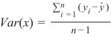
方差 (Variance)

​

其中 y_i 是单个目标特征值，bary 是这些目标特征值的平均值。

以上面为例，Price_of_Sale 目标特征的总方差计算如下：

= \(19.903125 \times 10^9 \quad \text{# 很大的数字 ;) \text{但这不影响我们的计算}\)

由于我们想知道哪个描述性特征最适合用于分割目标特征，我们必须计算描述性特征的每个值相对于目标特征值的方差。

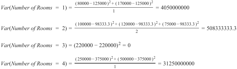
因此，对于上面的 Number_of_Rooms 描述性特征，我们得到单个房间数量的方差：

由于我们现在还想解决某些特征值出现频率相对较低但方差较高的问题（这可能导致整个特征的方差非常高，仅仅因为一个离群的特征值，即使所有其他特征值的方差可能很小），我们通过计算每个特征值的加权方差来解决这个问题：

最后，我们将这些加权方差相加，以对整个特征进行评估：

在我们的例子中是：

1012500000+190625000+0+7812500000=9015625000

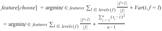
将所有这些结合起来，最终得到了我们将用于分裂过程中每个节点以确定下一个应该选择哪个特征来分割数据集的加权特征方差公式。

​

这里，f 表示单个特征，l 表示特征的值（例如 Price == medium），t 表示子集中目标特征的值，其中 f=l。

---

按照这个计算规范，我们可以在每个节点找到要分割数据集的特征。

为了说明沿最低方差特征值分割数据集的过程，我们以 UCI 自行车共享数据集的简化示例为例，我们将在本章的“从头开始用 Python 实现回归树”部分中使用该数据集，并计算每个特征的方差以找到我们应该用作根节点的特征。

Python

import pandas as pd
df = pd.read_csv("data/day.csv", usecols=['season','holiday','weekday','weathersit','cnt'])
df_example = df.sample(frac=0.012)

# 以下是示例计算，实际输出会依赖于 df_example 的随机样本
# 假设 df_example 包含以下数据，以便于理解计算过程
# season: 1, 1, 2, 3, 3, 4, 4, 4, 4
# cnt: 352, 421, 12, 162, 112, 161, 109, 79, 79

# 这里给出的计算是加权方差的近似值，具体值取决于df_example中的实际数据
# 为了演示概念，以下是根据原文提供的输出格式进行的推断：

# Season (假设 Season 有4个唯一值，以及它们对应的cnt均值和数据点数量)
# 例如：
# Season 1: cnts = [352, 421], mean = 386.5
# Season 2: cnts = [12], mean = 12
# Season 3: cnts = [162, 112], mean = 137
# Season 4: cnts = [161, 109, 79, 79], mean = 107
# n (total samples) = 9

# WeightVar(Season) = (2/9) * Var(Season=1_cnts) + (1/9) * Var(Season=2_cnts) + ...
# 原文提供了一个简化值：
# WeightVar(Season) = 16429.1

# Weekday (假设 Weekday 有多个唯一值，以及它们对应的cnt均值和数据点数量)
# 例如：
# Weekday 1: cnts = [109, 79], mean = 94
# Weekday 2: cnts = [162, 112], mean = 137
# Weekday 3: (no instance in example)
# Weekday 4: cnts = [421], mean = 421
# Weekday 5: cnts = [161], mean = 161
# n (total samples) = 9

# WeightVar(Weekday) = (2/9) * Var(Weekday=1_cnts) + (2/9) * Var(Weekday=2_cnts) + ...
# 原文提供了一个计算格式，没有最终值，但假设它会很小

# Weathersit (假设 Weathersit 有多个唯一值，以及它们对应的cnt均值和数据点数量)
# 例如：
# Weathersit 1: cnts = [421, 165, 12, 161, 112], mean = 174.2
# Weathersit 2: cnts = [352, 109], mean = 230.5
# n (total samples) = 9

# WeightVar(Weathersit) = (5/9) * Var(Weathersit=1_cnts) + (2/9) * Var(Weathersit=2_cnts) + ...
# 原文提供了一个计算格式，没有最终值，但假设它会比较大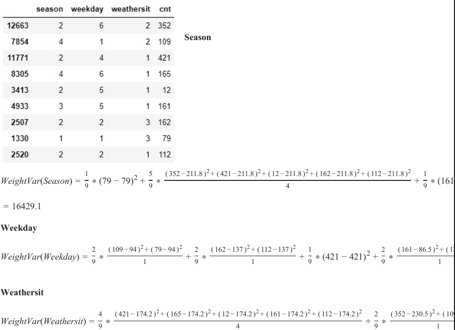

由于 Weekday 特征的方差最低，因此该特征用于分割数据集，并因此充当根节点。尽管由于随机抽样，此示例不够健壮（例如，没有 weekday == 3 的实例），但它应该传达使用方差作为分裂度量的数据分割背后的概念。

---

既然我们已经介绍了如何使用方差度量来分割具有连续目标特征的数据集的概念，我们现在将调整分类树的伪代码，以便我们的树模型能够处理连续尺度的目标特征值。

如上所述，我们需要进行两项更改，以使我们的树模型能够处理连续尺度的目标特征值：

1. 我们引入一个早期停止标准**，规定如果节点处的实例数量小于或等于 5（我们可以调整此值），则返回这些数字的平均目标特征值。**

2. 我们不再使用信息增益**，而是使用特征的方差作为新的分裂标准。**

因此，伪代码变为：

ID3(D, Feature_Attributes, Target_Attributes, min_instances=5)

创建根节点 r
将 r 设置为 D 中目标特征值的**平均值** ####### 已更改 ########

如果 num_instances <= min_instances :
    返回 r
否则:
    继续

如果 Feature_Attributes 为空:
    返回 r
否则:
    Att = Feature_Attributes 中**加权方差最低**的属性 ####### 已更改 ########
    r = Att

对于 Att 中的每个值:
    在 r 下添加一个新节点，其中 node_values = (Att == values)
    Sub_D_values = (Att == values)

    如果 Sub_D_values == empty:
        添加一个叶节点 l，其中 l 等于 D 中目标值的**平均值**
    否则:
        添加子树，使用 ID3(Sub_D_values, Feature_Attributes = Feature_Attributes 中去除 Att 的属性, Target_Attributes, min_instances=5)

除了实际算法中的更改，我们还必须使用另一种准确性度量，因为我们不再处理分类目标特征值。也就是说，我们不能再简单地将预测的类别与真实的类别进行比较，并计算命中目标的百分比。相反，我们使用均方根误差 (RMSE) 来衡量我们模型的“准确性”。

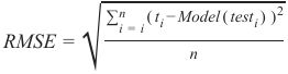
RMSE 的公式为：

​

其中 \(t_i\) 是测试数据集的实际测试目标特征值，Model(\(test_i\)) 是我们训练的回归树模型对这些 \(t_i\) 预测的值。通常，RMSE 值越低，我们的模型越符合实际数据。

既然我们已经调整了我们主要的 ID3 分类树算法以处理连续尺度的目标特征，并将其转变为回归树模型，我们就可以开始在 Python 中实现这些更改了。

因此，我们只需从前一章中获取分类树模型，并实现上述两项更改。

As stated above, the task during growing a Regression Tree is in principle the same as during the creation of
Classification Trees. Though, since the IG turned out to be no longer an appropriate splitting criteria (neither is
the Gini Index) due to the continuous character of the target feature we must have a new splitting criteria.
Therefore we use the variance which we will introduce now.
Variance
∑ n
 ( y − y ˉ )
ii =1
Var(x) =
n −1
Where y are the single target feature values and y ˉ is the mean of these target feature values.
iTaking the example from above the total variance of the Prize_of_Sale target feature is calculated with:
( 100000 − 189375 )2 + ( 120000 − 189375 ) 2 + ( 250000 − 189375 ) 2 + ( 80000 − 189375 )2 + ( 220000 − 189375 ) 2 + ( 170000 − 18
Var(Price of Sale) =
7
= 19.903125 ∗ 10 9 #Large Number ;) Though this has no effect on our calculations
Since we want to know which descriptive feature is best suited to split the target feature on, we have to
calculate the variance for each value of the descriptive feature with respect to the target feature values.
Hence for the Number_of_Rooms descriptive feature above we get for the single numbers of rooms:
( 80000 − 125000 )2 + ( 170000 − 125000 )2
Var(Number of Rooms = 1) =
 = 4050000000
1
( 100000 − 98333.3 ) 2 + ( 120000 − 98333.3 ) 2 + ( 75000 − 98333.3 ) 2
Var(Number of Rooms = 2) =
 = 508333333.3
2
Var(Number of Rooms = 3) = (220000 − 220000) 2 = 0
( 250000 − 375000 ) 2 + ( 500000 − 375000 ) 2
Var(Number of Rooms = 4) =
 = 31250000000
1
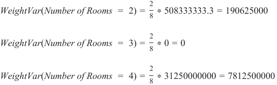
Since we now want to also address the issue that there are feature values which occur relatively rarely but
have a high variance (This could lead to a very high variance for the whole feature just because of one outliner
feature value even though the variance of all other feature values may be small) we address this by calculating
the weighted variance for each feature value with:
2
WeightVar(Number of Rooms = 1) = ∗ 4050000000 = 1012500000
8418
2
WeightVar(Number of Rooms = 2) = ∗ 508333333.3 = 190625000
82
WeightVar(Number of Rooms = 3) = ∗ 0 = 0
82
WeightVar(Number of Rooms = 4) = ∗ 31250000000 = 7812500000
8Finally, we sum up these weighted variances to make an assessment about the feature as a whole:
SumVar(feature) = ∑ value ∈ featureWeightVar(feature value)
Which is in our case:
1012500000 + 190625000 + 0 + 7812500000 = 9015625000
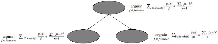
Putting all this together finally leads to the formula for the weighted feature variance which we will use at
each node in the splitting process to determine which feature we should choose to split our dataset on next.
| f = l |
feature[choose] = argminf ∈ features ∑ l ∈ levels ( f ) | f | ∗ Var(t, f = l)
∑n
 ( t − t ˉ ) 2
| f = l |
 i = 1
 i= argminf ∈ features ∑ l ∈ levels ( f ) | f | ∗
 n −1
Here f denotes a single feature, l denotes the value of a feature (e.g Price == medium), t denotes the value of
the target feature in the subset where f=l.
Following this calculation specification we find the feature at each node to split our dataset on.
419
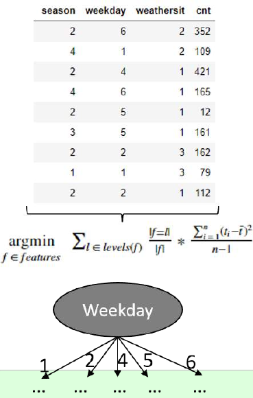
To illustrate the process of splitting the dataset along the feature values of the lowest variance feature, we take
a simplified example of the UCI bike sharing dataset which we will use later on in the Regression Trees from
scratch with Python part of this chapter and calculate the variance for each feature to find the feature we
should use as root node.
import pandas as pd
df = pd.read_csv("data/day.csv",usecols=['season','holiday','weekd
ay','weathersit','cnt'])
df_example = df.sample(frac=0.012)
Season
1
 5
 ( 352 − 211.8 ) 2 + ( 421 − 211.8 )2 + ( 12 − 211.8 )2 + ( 162 − 211.8 ) 2 + ( 112 − 211.8 ) 2
 1
WeightVar(Season) = ∗ (79 − 79) 2 + ∗
 + ∗ (161
9 9 4
 9= 16429.1
Weekday
2
 ( 109 − 94 ) 2 + ( 79 − 94 ) 2
 2
 ( 162 − 137 )2 + ( 112 − 137 )2
 1
 2
 ( 161 − 86.5 ) 2 + ( 12
WeightVar(Weekday) = ∗
 + ∗
 + ∗ (421 − 421) 2 +
 ∗
9 1
 9 1
 9
 9
 1
Weathersit
4
 ( 421 − 174.2 )2 + ( 165 − 174.2 )2 + ( 12 − 174.2 ) 2 + ( 161 − 174.2 ) 2 + ( 112 − 174.2 ) 2
 2
 ( 352 − 230.5 ) 2 + ( 109
WeightVar(Weathersit) = ∗
 + ∗
9 4
 9 1
Since the Weekday feature has the lowest variance, this feature is used to split the dataset on and hence serves
as root node. Though due to random sampling, this example is not that robust (for instance there is no instance
420
with weekday == 3) it should convey the concept behind the data splitting using variance as splitting measure.
Since we now have introduced the concept of how the
measure of variance can be used to split a dataset with a
continuous target feature, we will now adapt the pseudocode
for Classification Trees such that our tree model is able to
handle continuously scaled target feature values.
As stated above, there are two changes we have to make to
enable our tree model to handle continuously scaled target
feature values:
**1. We introduce an early stopping criteria where we say
that if the number of instances at a node is ≤ 5 (we can
adjust this value), return the mean target feature value of
these numbers**
**2. Instead of the information gain we use the variance of a
feature as our new splitting criteria**
Hence the pseudocode becomes:
ID3(D,Feature_Attributes,Target_Attr
ibutes,min_instances=5)
Create a root node r
Set r to the mean of the target feature values in D #######Cha
nged########
If num_instances <= min_instances :
return r
Else:
pass
If Feature_Attributes is empty:
return r
Else:
Att = Attribute from Feature_Attributes with the lowest we
ighted variance ########Changed########
r = Att
For values in Att:
Add a new node below r where node_values = (Att == val
ues)
421
Sub_D_values = (Att == values)
If Sub_D_values == empty:
Add a leaf node l where l equals the mean of the t
arget values in D
Else:
add Sub_Tree with ID3(Sub_D_values,Feature_Attribu
tes = Feature_Attributes without Att, Target_Attributes,min_instan
ces=5)
In addition to the changes in the actual algorithm we also have to use another measure of accuracy because we
are no longer dealing with categorical target feature values. That is, we can no longer simply compare the
predicted classes with the real classes and calculate the percentage where we bang on the target. Instead we are
using the root mean square error (RMSE) to measure the "accuracy" of our model.
The equation for the RMSE is:
RMSE =
 √
 ∑ n
 i = i
 ( t i − Model n
 ( test i ) )2
Where t i are the actual test target feature values of a test dataset and Model(test i) are the values predicted by
our trained regression tree model for these t i. In general, the lower the RMSE value, the better our model fits
the actual data.
Since we now have adapted our principal ID3 classification tree algorithm to handle continuously scaled target
features and therewith have made it to a regression tree model, we can start implementing these changes in
Python.
Therefore we simply take the classification tree model from the previous chapter and implement the two
changes mentioned above.