在Python中从头开始回归决策树(Regression Decision Trees from scratch in Python)
章节大纲
-
正如我们之前宣布的,为了实现我们的回归树模型,我们将使用 UCI 自行车共享数据集。我们将使用全部 731 个实例以及原始 16 个属性的子集。我们使用的属性是以下特征:
{'season', 'holiday', 'weekday', 'workingday', 'weathersit', 'cnt'},其中{'cnt'}特征作为我们的目标特征,表示每天租用自行车的总数。数据集的前五行如下所示:
Pythonimport pandas as pd dataset = pd.read_csv("data/day.csv",usecols=['season','holiday','weekday','workingday','weathersit','cnt']) dataset.sample(frac=1).head()Output:
     season  holiday  weekday  workingday  weathersit   cnt
458       2        0        2           1           1  6772
245       3        0        6           0           1  4484
86        2        0        1           1           1  2028
333       4        0        3           1           1  3613
507       2        0        2           1           2  6073
现在我们将开始修改原始创建的分类算法。有关代码的进一步注释,请读者参考前面关于分类树的章节。
所需 Python 包的导入 (Imports of Python Packages Needed)
Pythonimport pandas as pd import numpy as np from pprint import pprint import matplotlib.pyplot as plt from matplotlib import style style.use("fivethirtyeight") # 导入数据集并定义特征和目标列 dataset = pd.read_csv("data/day.csv",usecols=['season','holiday','weekday','workingday','weathersit','cnt']).sample(frac=1) mean_data = np.mean(dataset.iloc[:,-1])
方差计算函数 (Calculate the Variance of a Dataset)
Python""" 计算数据集的方差。 此函数接受三个参数。 1. data = 应该计算其特征方差的数据集 2. split_attribute_name = 应该计算其加权方差的特征名称 3. target_name = 目标特征的名称。此示例默认为 "cnt" """ def var(data,split_attribute_name,target_name="cnt"): feature_values = np.unique(data[split_attribute_name]) feature_variance = 0 for value in feature_values: # 创建数据子集 --> 沿 split_attribute_name 特征的值分割原始数据 # 并重置索引,以避免在使用 df.loc[] 操作时出现错误 subset = data.query('{0}=={1}'.format(split_attribute_name,value)).reset_index() # 计算每个子集的加权方差 # ddof=1 用于计算样本方差,即除以 n-1 value_var = (len(subset)/len(data))*np.var(subset[target_name],ddof=1) # 计算特征的加权方差 feature_variance+=value_var return feature_variance
分类算法 (Classification Algorithm)
Pythondef Classification(data,originaldata,features,min_instances,target_attribute_name,parent_node_class = None): """ 分类算法:此函数接受与前一章中原始分类算法相同的 5 个参数, 外加一个参数 (min_instances),它定义了每个节点的最小实例数作为早期停止标准。 """ # 定义停止条件 --> 如果满足其中一个条件,我们希望返回一个叶节点 ######### 此条件是新的 ######### # 如果所有 target_values 具有相同的值(对于分类),此处应返回目标特征的平均值 if len(data) <= int(min_instances): return np.mean(data[target_attribute_name]) ####################################################### # 如果数据集为空,返回原始数据集中的目标特征平均值 elif len(data)==0: return np.mean(originaldata[target_attribute_name]) # 如果特征空间为空,返回直接父节点的平均目标特征值 --> 注意,直接父节点是调用当前算法运行的节点, # 因此平均目标特征值存储在 parent_node_class 变量中。 elif len(features) ==0: return parent_node_class # 如果以上条件均不成立,则生长树! else: # 设置此节点的默认值 --> 当前节点的平均目标特征值 parent_node_class = np.mean(data[target_attribute_name]) # 选择最能分割数据集的特征 item_values = [var(data,feature) for feature in features] # 返回数据集中特征的方差 best_feature_index = np.argmin(item_values) best_feature = features[best_feature_index] # 创建树结构。根节点获取方差最小的特征 (best_feature) 的名称。 tree = {best_feature:{}} # 从特征空间中移除方差最小的特征 features = [i for i in features if i != best_feature] # 为根节点特征的每个可能值生长一个分支 for value in np.unique(data[best_feature]): value = value # 沿方差最小的特征值分割数据集,从而创建子数据集 sub_data = data.where(data[best_feature] == value).dropna() # 使用新参数为每个子数据集调用分类算法 --> 递归在此处体现! subtree = Classification(sub_data,originaldata,features,min_instances,'cnt',parent_node_class = parent_node_class) # 将从子数据集生长的子树添加到根节点下的树中 tree[best_feature][value] = subtree return tree
预测查询实例 (Predict Query Instances)
Pythondef predict(query,tree,default = mean_data): for key in list(query.keys()): if key in list(tree.keys()): try: result = tree[key][query[key]] except KeyError: # 捕获 KeyError 以处理未在训练数据中出现的新值 return default # 这里的 result = tree[key][query[key]] 是重复的,可以删除一个 # result = tree[key][query[key]] if isinstance(result,dict): return predict(query,result) else: return result
创建训练集和测试集 (Create Training and Testing Set)
Pythondef train_test_split(dataset): # 我们丢弃索引并重新标记索引,从 0 开始,因为我们不想在行标签/索引方面遇到错误 training_data = dataset.iloc[:int(0.7*len(dataset))].reset_index(drop=True) testing_data = dataset.iloc[int(0.7*len(dataset)):].reset_index(drop=True) return training_data,testing_data training_data = train_test_split(dataset)[0] testing_data = train_test_split(dataset)[1]
计算 RMSE (Compute the RMSE)
Pythondef test(data,tree): # 通过简单地从原始数据集中删除目标特征列并将其转换为字典来创建新的查询实例 queries = data.iloc[:,:-1].to_dict(orient = "records") # 创建一个空 DataFrame,其列中存储树的预测 predicted = [] # 计算 RMSE for i in range(len(data)): predicted.append(predict(queries[i],tree,mean_data)) RMSE = np.sqrt(np.sum(((data.iloc[:,-1]-predicted)**2)/len(data))) return RMSE
训练树、打印树和预测准确性 (Train the Tree, Print the Tree and Predict the Accuracy)
Pythontree = Classification(training_data,training_data,training_data.columns[:-1],5,'cnt') pprint(tree) print('#'*50) print('Root mean square error (RMSE): ',test(testing_data,tree))Output:
{'season': {1: {'weathersit': {1.0: {'workingday': {0.0: {'holiday': {0.0:
{0.0: 2398.1071428571427,
6.0: 2398.1071428571427}},
{1.0: 3284.28,
1.0:
1.0: {'holiday': {0.0:
2.0: 3284.28,
3.0: 3284.28,
4.0: 3284.28,
5.0: 3284.28}}}}}},
2.0: {'holiday': {0.0: {'weekday': {0.0: 2581.0: 21865,
2.0: {'w
{1.0: 2140.6666666666665}},
3.0: {'w
{1.0: 2049.0}},
4.0: {'w
{1.0: 3105.714285714286}},
5.0: {'w
{1.0: 2844.5454545454545}},
6.0: {'w
{0.0: 1757.111111111111}}}},
1.0: 1040.0}},
3.0: 473.5}},
2: {'weathersit': {1.0: {'workingday': {0.0: {'weekday': {0.0:
{0.0: 5728.2}},
1.0:
6667,
5.0:
6.0:
{0.0: 6206.142857142857}}}},
1.0: {'holiday': {0.0:
{1.0: 5340.06,
2.0:3.0:4.0:5340.06,
5340.06,
5340.06,
5.0: 5340.06}}}}}},
2.0: {'holiday': {0.0: {'workingday': {0.0:
{0.0: 4737.0,
6.0: 4349.7692307692305}},
1.0:
{1.0: 4446.294117647059,
2.0: 4446.294117647059,
3.0: 4446.294117647059,
4.0: 4446.294117647059,
5.0: 5975.333333333333}}}}}},
3.0: 1169.0}},
3: {'weathersit': {1.0: {'holiday': {0.0: {'workingday': {0.0:
{0.0: 5715.0,
6.0: 5715.0}},
1.0:
{1.0: 6148.342857142857,
2.0: 6148.342857142857,
3.0: 6148.342857142857,
4.0: 6148.342857142857,
5.0: 6148.342857142857}}}},
1.0: 7403.0}},
2.0: {'workingday': {0.0: {'holiday': {0.0:
{0.0: 4537.5,
6.0: 5028.8}},
1.0:
1.0: {'holiday': {0.0:
{1.0: 6745.25,
2.0: 5222.4,
3.0: 5554.0,
4.0: 4580.0,
5.0: 5389.409090909091}}}}}},
3.0: 2276.0}},
4: {'weathersit': {1.0: {'holiday': {0.0: {'workingday': {0.0:
{0.0: 4974.772727272727,
6.0: 4974.772727272727}},
{1.0: 5174.906976744186,
1.0:
2.0: 5174.906976744186,
3.0: 5174.906976744186,
4.0: 5174.906976744186,
5.0: 5174.906976744186}}}},
1.0: 3101.25}},
2.0: {'weekday': {0.0: 3795.6666666666665,
1.0: 4536.0,
2.0: {'holiday': {0.0: {'w
{1.0: 4440.875}}}},
3.0: 5446.4,
4.0: 5888.4,
5.0: 5773.6,
6.0: 4215.8}},
3.0: {'weekday': {1.0: 1393.5,
2.0: 2946.6666666666665,
3.0: 1840.5,
6.0: 627.0}}}}}}
##################################################
Root mean square error (RMSE): 1623.9891244058906
RMSE 学习曲线绘制 (Plot the RMSE with Respect to the Minimum Number of Instances)
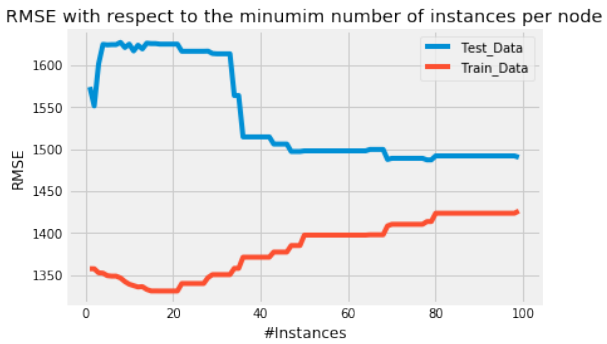
上面我们可以看到每个节点最少 5 个实例时的 RMSE。但目前,我们不知道这个结果是好是坏。为了了解我们模型的“准确性”,我们可以绘制一种学习曲线,其中我们绘制最小实例数与 RMSE 的关系。
Python""" 绘制 RMSE 与最小实例数的关系 """ fig = plt.figure() ax0 = fig.add_subplot(111) RMSE_test = [] RMSE_train = [] for i in range(1,100): tree = Classification(training_data,training_data,training_data.columns[:-1],i,'cnt') RMSE_test.append(test(testing_data,tree)) RMSE_train.append(test(training_data,tree)) ax0.plot(range(1,100),RMSE_test,label='Test_Data') ax0.plot(range(1,100),RMSE_train,label='Train_Data') ax0.legend() ax0.set_title('RMSE with respect to the minimum number of instances per node') ax0.set_xlabel('#Instances') ax0.set_ylabel('RMSE') plt.show()
最终回归树模型 (Final Regression Tree Model)
正如我们所看到的,增加每个节点的最小实例数会导致我们的测试数据的 RMSE 降低,直到我们达到大约每个节点 50 个实例。在这里,
Test_Data曲线趋于平坦,并且叶子中最小实例数的额外增加并不会显著降低我们测试集的 RMSE。让我们绘制一个最小实例数为 50 的树。
Pythontree = Classification(training_data,training_data,training_data.columns[:-1],50,'cnt') pprint(tree)Output:
{'season': {1: {'weathersit': {1.0: {'workingday': {0.0: 2407.5666666666666,
1.0: 3284.28}},
2.0: 2331.74,
3.0: 473.5}},
2: {'weathersit': {1.0: {'workingday': {0.0: 5850.178571428572,
1.0: 5340.06}},
2.0: 4419.595744680851,
3.0: 1169.0}},
3: {'weathersit': {1.0: {'holiday': {0.0: {'workingday': {0.0:
1.0:
{1.0: 5996.090909090909,
2.0: 6093.058823529412,
3.0: 6043.6,
4.0: 6538.428571428572,
5.0: 6050.2307692307695}}}},
1.0: 7403.0}},
2.0: 5242.617647058823,
3.0: 2276.0}},
4: {'weathersit': {1.0: {'holiday': {0.0: {'workingday': {0.0:
2727,
1.0:
4186}},
1.0: 3101.25}},
2.0: 4894.861111111111,
3.0: 1961.6}}}}
这就是我们最终的回归树模型。恭喜——大功告成!
As announced for the implementation of our regression tree model we will use the UCI bike sharing dataset
where we will use all 731 instances as well as a subset of the original 16 attributes. As attributes we use the
features: {'season', 'holiday', 'weekday', 'workingday', 'wheathersit', 'cnt'} where the {'cnt'} feature serves as
our target feature and represents the number of total rented bikes per day.
The first five rows of the dataset look as follows:
import pandas as pd
dataset = pd.read_csv("data/day.csv",usecols=['season','holida
y','weekday','workingday','weathersit','cnt'])
dataset.sample(frac=1).head()
Output:
season
holiday
weekday
workingday
weathersit
cnt
458
2
0
2
1
1
6772
245
3
0
6
0
1
4484
86
2
0
1
1
1
2028
333
4
0
3
1
1
3613
507
2
0
2
1
2
6073
We will now start adapting the originally created classification algorithm. For further comments to the code I
refer the reader to the previous chapter about Classification Trees.
"""
Make the imports of python packages needed
"""
import pandas as pd
import numpy as np
from pprint import pprint
import matplotlib.pyplot as plt
from matplotlib import style
423
style.use("fivethirtyeight")
#Import the dataset and define the feature and target columns#
dataset = pd.read_csv("data/day.csv",usecols=['season','holida
y','weekday','workingday','weathersit','cnt']).sample(frac=1)
mean_data = np.mean(dataset.iloc[:,-1])
##################################################################
#########################################
##################################################################
#########################################
"""
Calculate the varaince of a dataset
This function takes three arguments.
1. data = The dataset for whose feature the variance should be cal
culated
2. split_attribute_name = the name of the feature for which the we
ighted variance should be calculated
3. target_name = the name of the target feature. The default for t
his example is "cnt"
"""
def var(data,split_attribute_name,target_name="cnt"):
feature_values = np.unique(data[split_attribute_name])
feature_variance = 0
for value in feature_values:
#Create the data subsets --> Split the original data alon
g the values of the split_attribute_name feature
# and reset the index to not run into an error while usin
g the df.loc[] operation below
subset = data.query('{0}=={1}'.format(split_attribute_nam
e,value)).reset_index()
#Calculate the weighted variance of each subse
t
value_var = (len(subset)/len(data))*np.var(subset[target_n
ame],ddof=1)
#Calculate the weighted variance of the feature
feature_variance+=value_var
return feature_variance
##################################################################
424
#########################################
##################################################################
#########################################
def Classification(data,originaldata,features,min_instances,targe
t_attribute_name,parent_node_class = None):
"""
Classification Algorithm: This function takes the same 5 param
eters as the original classification algorithm in the
previous chapter plus one parameter (min_instances) which defi
nes the number of minimal instances
per node as early stopping criterion.
"""
#Define the stopping criteria --> If one of this is satisfie
d, we want to return a leaf node#
#########This criterion is new########################
#If all target_values have the same value, return the mean val
ue of the target feature for this dataset
if len(data) <= int(min_instances):
return np.mean(data[target_attribute_name])
#######################################################
#If the dataset is empty, return the mean target feature valu
e in the original dataset
elif len(data)==0:
return np.mean(originaldata[target_attribute_name])
#If the feature space is empty, return the mean target featur
e value of the direct parent node --> Note that
#the direct parent node is that node which has called the curr
ent run of the algorithm and hence
#the mean target feature value is stored in the parent_node_cl
ass variable.
elif len(features) ==0:
return parent_node_class
#If none of the above holds true, grow the tree!
else:
#Set the default value for this node --> The mean target f
eature value of the current node
parent_node_class = np.mean(data[target_attribute_name])
#Select the feature which best splits the dataset
item_values = [var(data,feature) for feature in features]
425
#Return the variance for features in the dataset
best_feature_index = np.argmin(item_values)
best_feature = features[best_feature_index]
#Create the tree structure. The root gets the name of the
feature (best_feature) with the minimum variance.
tree = {best_feature:{}}
#Remove the feature with the lowest variance from the feat
ure space
features = [i for i in features if i != best_feature]
#Grow a branch under the root node for each possible valu
e of the root node feature
for value in np.unique(data[best_feature]):
value = value
#Split the dataset along the value of the feature wit
h the lowest variance and therewith create sub_datasets
sub_data = data.where(data[best_feature] == value).dro
pna()
#Call the Calssification algorithm for each of those s
ub_datasets with the new parameters --> Here the recursion comes i
n!
subtree = Classification(sub_data,originaldata,feature
s,min_instances,'cnt',parent_node_class = parent_node_class)
#Add the sub tree, grown from the sub_dataset to the t
ree under the root node
tree[best_feature][value] = subtree
return tree
##################################################################
#########################################
##################################################################
#########################################
"""
426
Predict query instances
"""
def predict(query,tree,default = mean_data):
for key in list(query.keys()):
if key in list(tree.keys()):
try:
result = tree[key][query[key]]
except:
return default
result = tree[key][query[key]]
if isinstance(result,dict):
return predict(query,result)
else:
return result
##################################################################
#########################################
##################################################################
#########################################
"""
Create a training as well as a testing set
"""
def train_test_split(dataset):
training_data = dataset.iloc[:int(0.7*len(dataset))].reset_ind
ex(drop=True)#We drop the index respectively relabel the index
#starting form 0, because we do not want to run into errors re
garding the row labels / indexes
testing_data = dataset.iloc[int(0.7*len(dataset)):].reset_inde
x(drop=True)
return training_data,testing_data
training_data = train_test_split(dataset)[0]
testing_data = train_test_split(dataset)[1]
##################################################################
#########################################
##################################################################
#########################################
"""
Compute the RMSE
"""
427
def test(data,tree):
#Create new query instances by simply removing the target feat
ure column from the original dataset and
#convert it to a dictionary
queries = data.iloc[:,:-1].to_dict(orient = "records")
#Create a empty DataFrame in whose columns the prediction of t
he tree are stored
predicted = []
#Calculate the RMSE
for i in range(len(data)):
predicted.append(predict(queries[i],tree,mean_data))
RMSE = np.sqrt(np.sum(((data.iloc[:,-1]-predicted)**2)/len(dat
a)))
return RMSE
##################################################################
#########################################
##################################################################
#########################################
"""
Train the tree, Print the tree and predict the accuracy
"""
tree = Classification(training_data,training_data,training_data.co
lumns[:-1],5,'cnt')
pprint(tree)
print('#'*50)
print('Root mean square error (RMSE): ',test(testing_data,tree))
428
{'season': {1: {'weathersit': {1.0: {'workingday': {0.0: {'holiday': {0.0:
{0.0: 2398.1071428571427,
6.0: 2398.1071428571427}},
{1.0: 3284.28,
1.0:
1.0: {'holiday': {0.0:
2.0: 3284.28,
3.0: 3284.28,
4.0: 3284.28,
5.0: 3284.28}}}}}},
2.0: {'holiday': {0.0: {'weekday': {0.0: 258
1.0: 218
65,
2.0: {'w
{1.0: 2140.6666666666665}},
3.0: {'w
{1.0: 2049.0}},
4.0: {'w
{1.0: 3105.714285714286}},
5.0: {'w
{1.0: 2844.5454545454545}},
6.0: {'w
{0.0: 1757.111111111111}}}},
1.0: 1040.0}},
3.0: 473.5}},
2: {'weathersit': {1.0: {'workingday': {0.0: {'weekday': {0.0:
{0.0: 5728.2}},
1.0:
6667,
5.0:
6.0:
{0.0: 6206.142857142857}}}},
1.0: {'holiday': {0.0:
{1.0: 5340.06,
2.0:3.0:4.0:5340.06,
5340.06,
5340.06,
429
5.0: 5340.06}}}}}},
2.0: {'holiday': {0.0: {'workingday': {0.0:
{0.0: 4737.0,
6.0: 4349.7692307692305}},
1.0:
{1.0: 4446.294117647059,
2.0: 4446.294117647059,
3.0: 4446.294117647059,
4.0: 4446.294117647059,
5.0: 5975.333333333333}}}}}},
3.0: 1169.0}},
3: {'weathersit': {1.0: {'holiday': {0.0: {'workingday': {0.0:
{0.0: 5715.0,
6.0: 5715.0}},
1.0:
{1.0: 6148.342857142857,
2.0: 6148.342857142857,
3.0: 6148.342857142857,
4.0: 6148.342857142857,
5.0: 6148.342857142857}}}},
1.0: 7403.0}},
2.0: {'workingday': {0.0: {'holiday': {0.0:
{0.0: 4537.5,
6.0: 5028.8}},
1.0:
1.0: {'holiday': {0.0:
{1.0: 6745.25,
2.0: 5222.4,
3.0: 5554.0,
4.0: 4580.0,
5.0: 5389.409090909091}}}}}},
430
3.0: 2276.0}},
4: {'weathersit': {1.0: {'holiday': {0.0: {'workingday': {0.0:
{0.0: 4974.772727272727,
6.0: 4974.772727272727}},
{1.0: 5174.906976744186,
1.0:
2.0: 5174.906976744186,
3.0: 5174.906976744186,
4.0: 5174.906976744186,
5.0: 5174.906976744186}}}},
1.0: 3101.25}},
2.0: {'weekday': {0.0: 3795.6666666666665,
1.0: 4536.0,
2.0: {'holiday': {0.0: {'w
{1.0: 4440.875}}}},
3.0: 5446.4,
4.0: 5888.4,
5.0: 5773.6,
6.0: 4215.8}},
3.0: {'weekday': {1.0: 1393.5,
2.0: 2946.6666666666665,
3.0: 1840.5,
6.0: 627.0}}}}}}
##################################################
Root mean square error (RMSE): 1623.9891244058906
Above we can see RMSE for a minimum number of 5 instances per node. But for the time being, we have no
idea how bad or good that is. To get a feeling about the "accuracy" of our model we can plot kind of a learning
curve where we plot the number of minimal instances against the RMSE.
"""
Plot the RMSE with respect to the minimum number of instances
"""
fig = plt.figure()
ax0 = fig.add_subplot(111)
RMSE_test = []
RMSE_train = []
for i in range(1,100):
tree = Classification(training_data,training_data,training_dat
431
a.columns[:-1],i,'cnt')
RMSE_test.append(test(testing_data,tree))
RMSE_train.append(test(training_data,tree))
ax0.plot(range(1,100),RMSE_test,label='Test_Data')
ax0.plot(range(1,100),RMSE_train,label='Train_Data')
ax0.legend()
ax0.set_title('RMSE with respect to the minumim number of instance
s per node')
ax0.set_xlabel('#Instances')
ax0.set_ylabel('RMSE')
plt.show()
As we can see, increasing the minimum number of instances per node leads to a lower RMSE of our test data
until we reach approximately the number of 50 instances per node. Here the Test_Data curve kind of flattens
out and an additional increase in the minimum number of instances per leaf does not dramatically decrease the
RMSE of our testing set.
Lets plot the tree with a minimum instance number of 50.
tree = Classification(training_data,training_data,training_data.co
lumns[:-1],50,'cnt')
pprint(tree)
432
{'season': {1: {'weathersit': {1.0: {'workingday': {0.0: 2407.5666666666666
1.0: 3284.28}},
2.0: 2331.74,
3.0: 473.5}},
2: {'weathersit': {1.0: {'workingday': {0.0: 5850.178571428572,
1.0: 5340.06}},
2.0: 4419.595744680851,
3.0: 1169.0}},
3: {'weathersit': {1.0: {'holiday': {0.0: {'workingday': {0.0:
1.0:
{1.0: 5996.090909090909,
2.0: 6093.058823529412,
3.0: 6043.6,
4.0: 6538.428571428572,
5.0: 6050.2307692307695}}}},
1.0: 7403.0}},
2.0: 5242.617647058823,
3.0: 2276.0}},
4: {'weathersit': {1.0: {'holiday': {0.0: {'workingday': {0.0:
2727,
1.0:
4186}},
1.0: 3101.25}},
2.0: 4894.861111111111,
3.0: 1961.6}}}}
So thats our final regression tree model. Congratulations - Done!