Course: 11.3 最低广场 | The Way To Learn

Section outline

Select section General

Collapse Expand
General

Collapse all Expand all
- Select activity 新闻通告
  
  新闻通告 Forum

最小广场

You have calculated the linear correlation coefficient value $\begin{align*}r=-0.9542\end{align*}$ to determine that there is a strong linear relationship between the speed you drive and the gas you use. Suppose you want to predict the average MPG at a speed that you did not measure, like 85 mph. How could you use your research data (below) to provide an estimated value?
::您计算了线性相关系数值 r0. 9542, 以确定您驱动的速度与您使用的气体之间存在强烈的线性关系。如果您想要以您没有测量到的速度预测平均 MPG , 比如85 mph。您如何使用您的研究数据( 下面)来提供估计值 ?

MPG ::MPG MPG	25	24	22	22	19	14	11
MPH ::MPH 公共卫生和公共卫生部	45	50	55	60	65	70	75

Least Squares
::最小广场

The linear correlation coefficient $\begin{align*}r\end{align*}$ and coefficient of determination $\begin{align*}r^2\end{align*}$ can assist in determining the strength of a linear relationship between two variables, but are not helpful if you need to predict a value that has not been observed. In order to predict a value of a relationship, we need to find a line that represents the best average change in $\begin{align*}y\end{align*}$ based on change in $\begin{align*}x\end{align*}$ (you should recognize this as the slope of a line).
::线性相关系数 r 和 r2 确定系数 r 有助于确定两个变量之间线性关系的强度,但如果你需要预测一个未观察到的值,则无济于事。为了预测某种关系的价值,我们需要找到一条线,以 x 的变化为基础,代表y 的最佳平均变化(你应该承认这是一条线的斜坡)。

Consider the graph below:
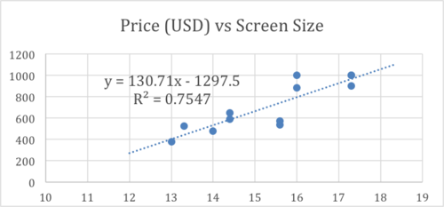
::考虑下图:

This scatterplot represents the price of laptops online related to screen size. The data points exhibit a clear positive trend, but are certainly not in a straight line. The $\begin{align*}r^2\end{align*}$ value of 0.755 suggests that approximately 75% of the increase in price as we move left to right may be attributed to the relationship between price and increased screen size.
::这个散射图代表了在线笔记本电脑与屏幕大小相关的价格。数据点呈现了明显的积极趋势,但肯定不是直线。 0.755的r2值表明,我们向右移动的价格上涨约75%可能归因于价格与屏幕大小增加之间的关系。

The dotted line $\begin{align*}y=130.71x-1297.5\end{align*}$ , drawn on the graph, is the line of best fit , calculated using the least squares method . The line of fit may be used to predict the likely values of price "> $\begin{align*}(y)\end{align*}$ , based on screen size $\begin{align*}(x)\end{align*}$ , for sizes not plotted on the graph. We can see just by looking that the estimated average price for a laptop with an 18″ screen size is about $1,075, and the estimated average price for a laptop with a 12″ screen is less than $300.
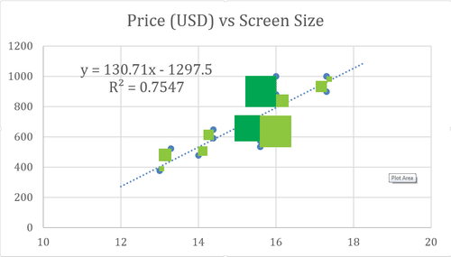
::在图上绘制的点线y=130.71x-1297.5是最适合的线,使用最小平方法计算。适合线可用于预测价格,根据屏幕大小(x),对于图形上没有绘制的大小。我们可以通过查看18英寸屏幕大小的笔记本电脑的估计平均价格约为1 075美元,而12英寸屏幕的笔记本电脑的估计平均价格不到300美元。

To understand what is meant by the least squares method, imagine a square formed from the distance of each point to the line. The square has four equal sides each equal to the shortest vertical distance between each point and the line, as illustrated below:
::为了理解最小方块方法的含义,请想象从每个点的距离到线之间的一个方块。如下文所示,该方块各有四个相等的方块,每方块等于每个点和线之间的最短垂直距离:

The line of best fit is the line resulting in the least total area of these squares. The line will always go through the point at the intersection of the mean $\begin{align*}x\end{align*}$ and mean $\begin{align*}y\end{align*}$ values: $\begin{align*}(\overline{x}, \overline{y})\end{align*}$ .
::最合适的线是导致这些方块总面积最小的线。该线将总是穿过平均值 x 和平均值 y 的交叉点x y ) 。

To identify the equation of the least squares line, you will need the following values calculated from your data:
::要确定最小方形线的方程式,需要从数据中计算以下数值:

$\begin{align*}\overline{x}\end{align*}$ : The mean value of $\begin{align*}x\end{align*}$ .
::x : x 的平均值。

$\begin{align*}\sigma_x\end{align*}$ or $\begin{align*}s_x\end{align*}$ : The standard deviation of the $\begin{align*}x\end{align*}$ values
::□x orsx: x 值的标准偏差

$\begin{align*}\overline{y}\end{align*}$ : The mean value of $\begin{align*}y\end{align*}$ .
::y:y的平均值。

$\begin{align*}\sigma_y\end{align*}$ or $\begin{align*}s_y\end{align*}$ : The standard deviation of the $\begin{align*}y\end{align*}$ values
::y orsy: Y 值的标准偏差

$\begin{align*}r\end{align*}$ : The linear correlation coefficient
::r:线性相关系数

Once you know this data, you can find the equation of the line of best fit in slope-intercept form $\begin{align*}Y=bX+a\end{align*}$ , with two easy formulas:
::一旦您知道这个数据, 您可以在斜坡界面的 Y=bX+a 中找到最适合的线的方程式, 有两个简单公式 :

\begin{aligned} b & = r (\frac{S_{y}}{S_{x}}) \\ a & = \bar{Y} - b \bar{X} \end{aligned}

$\begin{align*}b &=r \left(\frac{S_y}{S_x} \right)\\ a &=\overline{Y}-b \overline{X}\end{align*}$
::{\fn黑体\fs22\bord1\shad0\3aHBE\4aH00\fscx67\fscy66\2cHFFFFFF\3cH808080}Br(SySx)a=Y *bX* {\fn黑体\fs22\bord1\shad0\3aHBE\4aH00\fscx67\fscy66\2cHFFFFFF\3cH808080}Br(SySx)a=Y {\fn黑体\fs22\bord1\shad0\3aHBE\4aH00\fscx67\fscy66\2cHFFFFFF\3cH808080}

The least squares line is a powerful tool for predicting values, but the reliability of the predictions reduces as you get further from the observed data . Take care to recognize that any data point that you predict beyond the observed data carries an element of uncertainty that increases the further “out” you predict.
::最小的平方线线是预测数值的有力工具,但预测的可靠性会随着你从观察到的数据中走得更远而降低。请注意,您预测的超过观察到的数据的任何数据点都含有不确定因素,会增加您预测的“ 出局” 。

Finding the Line of Best Fit
::寻找最合适的线

Find the equation of the line of best fit given $\begin{align*}\overline{X}=13\end{align*}$ , $\begin{align*}\overline{Y}=6\end{align*}$ , $\begin{align*}s_x=4\end{align*}$ , $\begin{align*}s_y=1.5\end{align*}$ , and $\begin{align*}r=0.65\end{align*}$ .
::给 X = 13, Y = 6, sx= 4, sy= 1. 5, 和 r= 0. 65, 找到最适合的线的方程式。

To find the equation of the line, we need to calculate $\begin{align*}b\end{align*}$ , and $\begin{align*}a\end{align*}$ to substitute into the equation $\begin{align*}Y=bX+a\end{align*}$ :
::要找到线条的方程, 我们需要计算 b, 并替换为 Y=bX+a 的方程 :

$\begin{align*}b=r \left(\frac{s_y}{s_x} \right) \rightarrow b=0.65 \left(\frac{1.5}{4} \right)=0.65 \times 0.375 \approx 0.244\end{align*}$
::b=r (sysx) b=0.65(1.54)=0.65x0.3750.244

$\begin{align*}a=\overline{Y}-b \overline{X} \rightarrow a=6-0.244(13)=6-3.172 \approx 2.83\end{align*}$
::a=Y bX a=6-0.244(13)=6-3.1.722.83

Now we have $\begin{align*}a\end{align*}$ and $\begin{align*}b\end{align*}$ , we just substitute them into the equation:
::现在,我们有一个和B, 我们只是代之以他们的方程:

\begin{aligned} Y = 0.244 X + 2.83 \end{aligned}

$\begin{align*}Y=0.244X+2.83\end{align*}$
::Y=0.244X+2.83

Graphing and Finding the Line of Best Fit
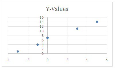
::划定和寻找最佳合适的线

Graph and find the equation of the line of best fit given the data from the following table:
::根据下表的数据,图表并查找最适合线的方程式:

$\begin{align}X\end{align}$ ::X 十	$\begin{align}Y\end{align}$ ::Y Y Y
-3	1
-1	4
0	7
3	11
5	14

Let’s graph the data first, using a scatter plot :
::让我们先用散射图绘制数据图:

Now we need to calculate our required values, as listed in the lesson:
::现在我们需要计算我们所需要的值, 正如课程中列出的:

$\begin{align*}\overline{X}: \frac{-3-1+0+3+5}{5}=0.80\end{align*}$
::X: - 3 - 1+0+3+55=0. 80

$\begin{align*}\sigma_x\end{align*}$ or $\begin{align*}s_x:=\sqrt{\left(\frac{(-3-0.8)^2+(-1-0.8)^2+(0-0.8)^2+(3-0.8)^2+(5-0.8)^2}{5-1} \right)}=3.19\end{align*}$
::xorsx:= ((-3-0.8)2+(-1-0.8)2+(-0-0.8)2+(0-0.8)2+(3-0.8)2+(5-0.8)2+(5-0.8)25-1=3.19

$\begin{align*}\overline{Y}: -7.4\end{align*}$
::你: - 7.4

$\begin{align*}\sigma_y\end{align*}$ or $\begin{align*}s_y: =5.225\end{align*}$
::食道:=5.225

$\begin{align*}r: = 0.9948\end{align*}$ (calculated using the online tool at NCAL Calculator's website ).
::r:0.9948(使用NCAL计算器网站的在线工具计算)。

Now we can use our two new formulas to find $\begin{align*}a\end{align*}$ and $\begin{align*}b\end{align*}$ :
::现在我们可以用我们的两个新公式来找到一个和b:

$\begin{align*}b=r \left(\frac{s_y}{s_x} \right) \rightarrow b=0.9948 \left(\frac{5.225}{3.19} \right) \approx 0.9948 (1.638) \approx 1.63\end{align*}$
::b=r (sysx) b=0.9948 (5.2253.19) 0.9948 (1.638) 1.63

$\begin{align*}a=\overline{Y}-b \overline{X} \rightarrow -7.4-1.63(0.80)=-7.4-1.304=-8.704\end{align*}$
::a=Y bX 7.4-1.63(0.80)7.4-1.3048.704

The equation of the line of best fit is: $\begin{align*}Y=1.63X-8.704\end{align*}$
::最合适线的等式是:Y=1.63X-8.704

Real-World Application: Grocery Shopping
::真实世界应用程序: 杂草购物

Pandi is shopping for rice at her local supermarket, and notes that the rice comes in different size packages, 6 oz for $1.75, 12 oz for $3.50, 18 oz for $4.68, 28 oz for $7.90, 44 oz for $13.09 and the “Family Size” package of 64 oz that has no price listed. If Pandi wants the Family Size package, what price would you predict it sells for?
::Pandi在本地超市购买大米,并指出大米的尺寸不同,每米6美元,每米1.75美元,每米12美元,每米3.50美元,每米18美元,每米4.68美元,每米28美元,每米7.90美元,每米13.09美元,每米44美元,每米64美元,没有价格。如果Pandi想要家庭大小一揽子计划,你预测它卖出多少价格?

First we need to find the equation of best fit, just as we did in Example B.
::首先,我们需要找到最合适的方程式,就像我们在例B中所做的那样。

Necessary values:
::必要值:

$\begin{align*}\overline{X}: 21.6\end{align*}$
::X : 21.6

$\begin{align*}\sigma_{x}\end{align*}$ or $\begin{align*}s_x: = 14.9265\end{align*}$
::x或 sx:=14.9265

$\begin{align*}\overline{Y}: 6.184\end{align*}$
::你:6.184

$\begin{align*}\sigma_{y}\end{align*}$ or $\begin{align*}s_y: =4.4655\end{align*}$
::y :=4.4655

$\begin{align*}r: = 0.9978\end{align*}$ (Calculated online at NCAL Calculator's website).
::r: r=0.9978(通过NCAL计算器网站在线计算)。

Finding $\begin{align*}a\end{align*}$ and $\begin{align*}b\end{align*}$ :
::查找 a 和 b:

$\begin{align*}b=r \left(\frac{s_y}{s_x} \right) \rightarrow b=0.9978 \left(\frac{4.4655}{14.9265} \right) \approx 0.299\end{align*}$
::b=r (sysx) b= 0.9978 (4.4665514.9265) 0.299

$\begin{align*}a=\overline{Y}-b \overline{X} \rightarrow 6.184-0.299(21.6)=-0.2744\end{align*}$
::a=Y bX 6.184-0.299(21.6)0.2744

The equation of the line of best fit is: $\begin{align*}Y=0.299x-0.2744\end{align*}$

::最合适线的等式是:Y=0.299x-0.2744

Now that we have an equation for the line of fit, we can just substitute in the $\begin{align*}x\end{align*}$ -value of 64 oz to calculate a predicted price:
::现在我们有了适合线的方程式, 我们可以用64oz的x值来替代, 来计算一个预测价格:

\begin{aligned} Y & = 0.299 (64) - 0.2744 \\ Y & = 19.135 - 0.2744 \\ Y & \approx $ 18.86 \end{aligned}

$\begin{align*}Y &=0.299(64)-0.2744 \\ Y &=19.135-0.2744 \\ Y & \approx \$ 18.86\end{align*}$
::Y=0.299(64)-0.2744Y=19135-0.2744Y=18.86美元

Earlier Problem Revisited
::重审先前的问题

You have calculated the linear correlation coefficient value $\begin{align*}r=-0.9542\end{align*}$ to determine that there is a strong linear relationship between the speed you drive and the gas you use. Suppose you want to predict the average MPG at a speed that you did not measure, like 85 mph. How could you use your research data (below) to provide an estimated value?
::您已经计算了线性相关系数值 r0. 9542, 以确定您驱动的速度与您使用的气体之间存在强烈的线性关系。如果您想要以您没有测量到的速度预测平均 MPG , 比如85 mph。您如何使用您的研究数据( 下面)来提供估计值 ?

MPG ::MPG MPG	25	24	22	22	19	14	11
MPH ::MPH 公共卫生和公共卫生部	45	50	55	60	65	70	75

This is very much like Example C, we need to find the equation of best fit, and then substitute 85 mph in for $\begin{align*}X\end{align*}$ to find the predicted MPG.
::这与例C非常相似, 我们需要找到最合适的方程式, 然后用85mph 替换X 来找到预测的MPG。

Let’s use the online tool at NCAL Calculator's website to find our necessary data:
::让我们使用NCAL计算器网站的在线工具找到我们必要的数据:

$\begin{align*}\overline{X}: 60\end{align*}$
::X : 60

$\begin{align*}\sigma_x\end{align*}$ or $\begin{align*}s_x:=10.8012\end{align*}$
::x orsx:=10.8012

$\begin{align*}\overline{Y}: 19.57\end{align*}$
::你: 19. 57

$\begin{align*}\sigma_{y}\end{align*}$ or $\begin{align*}s_y: =5.2554\end{align*}$
::y := 5.2554

$\begin{align*}r: = -0.9542\end{align*}$
::r: r: 0.9542

$\begin{align*}b=r \left(\frac{s_y}{s_x} \right) \rightarrow b=-0.9542 \left(\frac{5.2554}{10.8012} \right) \approx -0.464 \end{align*}$
::b=r (sysx) b 0.9542(5.25554.10.8012) 0.464

$\begin{align*}a=\overline{Y}-b \overline{X} \rightarrow 19.57+0.464(60)=47.41\end{align*}$
::a=Y bX 19.57+0.464(60)=47.41

The equation of the line of best fit is: $\begin{align*}Y=-0.464X+47.41\end{align*}$

::最合适线的等式是:Y0.464X+47.41。

Substituting 85 in for $\begin{align*}X\end{align*}$ yields:
::X产量替代85分:

\begin{aligned} Y & = - 0.464 (85) + 47.41 \\ Y & = 7.97 \end{aligned}

$\begin{align*}Y &=-0.464(85)+47.41 \\ Y &=7.97\end{align*}$
::Y0.464(85)+47.41Y=7.97

At 85 mph, we predict the fuel efficiency to be 7.97 mpg.
::在85英里时,我们预测燃料效率为7.97兆克。

Examples
::实例

Examples 1-5 use the following data:
::实例1-5使用以下数据:

\begin{aligned} x_{1} & = 14.26, x_{2} = 12.82, x_{3} = 11.29, x_{4} = 10.02, and x_{5} = 9.71 \\ y_{1} & = 29.43, y_{2} = 34.92, y_{3} = 40.29, y_{4} = 46, and y_{5} = 49.78 \end{aligned}

$\begin{align*}x_1&=14.26, \ x_2=12.82, \ x_3=11.29, \ x_4=10.02, \text{ and } x_5=9.71\\ y_1&=29.43, \ y_2=34.92, \ y_3=40.29, \ y_4=46, \text{ and } y_5=49.78\end{align*}$
::x1=14.26, x2=12.82, x3=11.29, x4=10.02, x5=9.71y1=29.43, y2=34.92, y3=40.29, y4=46, y5=49.78

Example 1
::例1

What are the $\begin{align*}\mu\end{align*}$ and $\begin{align*}\sigma\end{align*}$ values for $\begin{align*}x\end{align*}$ and $\begin{align*}y\end{align*}$ ?
::x 和 y 的 μ 值和 □ 值是什么 ?

$\begin{align*}\mu_x=11.62\end{align*}$ , $\begin{align*}\mu_y=40.084\end{align*}$ , $\begin{align*}\sigma_x=1.918\end{align*}$ , and $\begin{align*}\sigma_y=8.204\end{align*}$
::μx=11.62, 微y=40.084, 1-13x=1.918, y=8.204

Example 2
::例2

What is the linear correlation coefficient?
::线性相关系数是多少?

$\begin{align*}r=-0.9906\end{align*}$
::r0.9906

Example 3
::例3

What is the equation of the line of best fit?
::最合适线的等式是什么?

$\begin{align*}b=-0.9906 \left(\frac{8.204}{1.918} \right)=-4.237 \end{align*}$
::b0.906(8.2041.918)4.237

Example 4
::例4

What would you predict $\begin{align*}y_6\end{align*}$ to be, if $\begin{align*}x_6=7.42\end{align*}$ ?
::如果x6=7.42,你预测y6会是什么?

$\begin{align*}Y_6=-4.237(7.42)+89.318\end{align*}$
::Y64.237(7.42)+89.318

$\begin{align*}Y_6=57.88\end{align*}$
::Y6=57.88

Example 5
::例5

What would you predict $\begin{align*}y_0\end{align*}$ to be, if $\begin{align*}x_0=16.28\end{align*}$ ?
::如果x0=16.28,你预测的Y0会是什么?

$\begin{align*}Y_0=-4.237(16.28)+89.318\end{align*}$
::YO4.237(16.28)+89.318

$\begin{align*}Y_0=20.34\end{align*}$
::Y0=20.34

Review
::回顾

1. What does the symbol $\begin{align*}\mu_x\end{align*}$ represent in the context of the lesson?
::1. 微x的符号在教训中代表什么?

2. What does the symbol $\begin{align*}\sigma_y\end{align*}$ represent in the context of the lesson?
::2. 该符号在教训中代表什么?

3. What does the symbol $\begin{align*}r\end{align*}$ represent in the context of the lesson?
::3. 在经验教训方面,符号r代表什么?

4. As compared to the standard slope-intercept form of an equation that you likely first learned about in Algebra I, what do $\begin{align*}a\end{align*}$ and $\begin{align*}b\end{align*}$ represent?
::4. 与你可能首先在代数一中了解到的标准斜度拦截方程式形式相比,a和b代表什么?

5. What is a line of best fit?
::5. 什么是最适合的一行?

6. What is meant by referring to the ‘least squares’?
::6. " 最小广场 " 是指什么?

Questions 7-11 refer to the following data:
::问题7-11涉及以下数据:

\begin{aligned} x_{1} = & 2, x_{2} = 4, x_{3} = 5, x_{4} = 8, and x_{5} = 11 \\ y_{1} = - 4, & y_{2} = - 7, y_{3} = - 9, y_{4} = - 12, and y_{5} = - 16 \end{aligned}

$\begin{align*}x_1 =& \ 2, \ x_2=4, \ x_3=5, \ x_4=8, \text{ and } x_5=11\\ y_1=-4, \ & y_2=-7, \ y_3=-9, \ y_4=-12, \text{ and } y_5=-16\end{align*}$
::x1= 2, x2=4, x3=5, x4=8, x5=11y1=8, x5=11y1=4, y24, y27, y39, y412, y516

7. What are the $\begin{align*}\mu\end{align*}$ and $\begin{align*}\sigma\end{align*}$ values for $\begin{align*}x\end{align*}$ and $\begin{align*}y\end{align*}$ ?
::7. x 和 y 的 μ 值和 □ 值是多少?

8. What is the linear correlation coefficient?
::8. 线性相关系数是多少?

9. What is the equation of the line of best fit?
::9. 最合适线的等式是什么?

10. What would you predict $\begin{align*}y_6\end{align*}$ to be, if $\begin{align*}x_6=14\end{align*}$ ?
::10. 如果x6=14,你预测y6会是什么?

11. What would you predict $\begin{align*}y_0\end{align*}$ to be, if $\begin{align*}x_0=0\end{align*}$ ?
::11. 如果x0=0,你预测Y0会是什么?

Questions 12-16 refer to the following:
::问题12-16涉及以下方面:

Brian wonders if more expensive skis slide better, and collects the following data:
::Brian想知道更昂贵的滑雪滑雪滑雪滑雪是否更好,并收集以下数据:

Ski Cost in USD ::滑雪成本(美元)	Sliding Coefficient ::滑滑系数
237.43	0.06
283.92	0.056
343.50	0.05
373.89	0.049
422.99	0.051
487.50	0.05
505.24	0.046

12. What are the $\begin{align*}\mu\end{align*}$ and $\begin{align*}\sigma\end{align*}$ values for $\begin{align*}x\end{align*}$ and $\begin{align*}y\end{align*}$ ?
::12. x 和 y 的 μ 和 □ 值是多少?

13. What is the linear correlation coefficient?
::13. 线性相关系数是多少?

14. What is the equation of the line of best fit?
::14. 最合适线的等式是什么?

15. What would you predict the sliding coefficient of a $650 pair of skis to be?
::15. 你会预测650美元雪橇滑动系数是多少?

16. How would you describe the relationship between price and sliding coefficient, based on Brian’s data?
::16. 根据Brian的数据,你如何描述价格和滑动系数之间的关系?

Review (Answers)
::回顾(答复)

Click to see the answer key or go to the Table of Contents and click on the Answer Key under the 'Other Versions' option.
::单击可查看答题键, 或转到目录中, 单击“ 其他版本” 选项下的答题键。

Section outline

General

最小广场

Least Squares ::最小广场

Finding the Line of Best Fit ::寻找最合适的线

Graphing and Finding the Line of Best Fit ::划定和寻找最佳合适的线

Real-World Application: Grocery Shopping ::真实世界应用程序: 杂草购物

Earlier Problem Revisited ::重审先前的问题

Examples ::实例

Example 1 ::例1

Example 2 ::例2

Example 3 ::例3

Example 4 ::例4

Example 5 ::例5

Review ::回顾

Review (Answers) ::回顾(答复)