机器学习
瓦普尼克-切尔沃宁基斯维数(VC 维)和概率近似正确(PAC)学习是可学习性数学理论中两个重要的概念,因此它们都具有数学导向性。前者衡量的是分类算法可以学习的函数空间的容量(复杂性、表达能力、丰富性或灵活性)。它最初由 Vladimir Vapnik 和 Alexey Chervonenkis 于 1971 年定义。后者是学习算法数学分析的框架。目标是检查所选假设近似正确的概率是否非常高。PAC 学习的概念由 Leslie Valiant 于 1984 年提出。
VC 维
设 H 为某个机器学习问题的假设空间。H 的瓦普尼克-切尔沃宁基斯维数,也称为 H 的 VC 维,记作 VC(H),是空间 H 的**复杂性(或容量、表达能力、丰富性或灵活性)的度量。为了定义 VC 维,我们需要集合的破碎(shattering)**概念。
集合的破碎
设 D 是一个包含 N 个示例的数据集,用于二元分类问题,类别标签为 0 和 1。设 H 是该问题的假设空间。H 中的每个假设 h 将 D 分为两个不相交的子集,如下所示:
D0={x∈D∣h(x)=0}
D1={x∈D∣h(x)=1}
这样的 D 的划分被称为“二分法”(dichotomy)。可以证明,D 中有 2N 种可能的二分法。对于 D 的每种二分法,都存在对 D 元素进行标签“1”和“0”的唯一分配。反之,如果 S 是 D 的任何子集,那么 S 定义了一个唯一的假设 h,如下所示: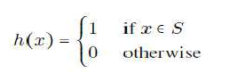
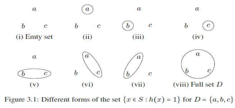
因此,为了指定一个假设 h,我们只需要指定集合 {x∈D∣h(x)=1}。图 3.1 显示了当 D 包含三个元素时 D 的所有可能二分法。在图中,我们只显示了二分法中的两个集合之一,即集合 {x∈D∣h(x)=1}。圆圈和椭圆表示这样的集合。
定义
如果对于 D 的每种二分法,在 H 中都存在某个与 D 的二分法一致的假设,则称一个示例集 D 被假设空间 H 破碎。
以下示例说明了瓦普尼克-切尔沃宁基斯维数的概念。
示例
在图中,我们看到一个轴对齐矩形可以破碎二维空间中的四个点。因此,当 H 是二维轴对齐矩形的假设类时,VC(H) 为四。在计算 VC 维时,只要我们能找到四个可以被破碎的点就足够了;我们没有必要能够破碎二维空间中的任意四个点。
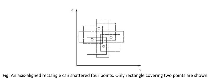
图:一个轴对齐矩形可以破碎四个点。只显示了覆盖两个点的矩形。
VC 维可能看起来有些悲观。它告诉我们,使用矩形作为我们的假设类,我们只能学习包含四个点的数据集,而不能更多。
The concepts of Vapnik-Chervonenkis dimension (VC dimension) and probably approximate
correct (PAC) learning are two important concepts in the mathematical theory of learnability and hence
are mathematically oriented. The former is a measure of the capacity (complexity, expressive power,
richness, or flexibility) of a space of functions that can be learned by a classification algorithm. It was
originally defined by Vladimir Vapnik and Alexey Chervonenkis in 1971. The latter is a framework for the
mathematical analysis of learning algorithms. The goal is to check whether the probability for a selected
hypothesis to be approximately correct is very high. The notion of PAC
learning was proposed by Leslie Valiant in 1984.
V-C dimension
Let H be the hypothesis space for some machine learning problem. The Vapnik-Chervonenkis dimension
of H, also called the VC dimension of H, and denoted by V C(H), is a measure of the complexity (or,
capacity, expressive power, richness, or flexibility) of the space H. To define the VC dimension we
require the notion of the shattering of a set of instances.
Shattering of a set
Let D be a dataset containing N examples for a binary classification problem with class labels 0 and 1.
Let H be a hypothesis space for the problem. Each hypothesis h in H partitions D into two disjoint
subsets as follows:
Such a partition of S is called a “dichotomy” in D. It can be shown that there are 2 N possible dichotomies
in D. To each dichotomy of D there is a unique assignment of the labels “1” and “0” to the elements of
D. Conversely, if S is any subset of D then, S defines a unique hypothesis h as follows:
Thus to specify a hypothesis h, we need only specify the set {x Є D | h(x) = 1}. Figure 3.1 shows all
possible dichotomies of D if D has three elements. In the figure, we have shown only one of the two sets
in a dichotomy, namely the set {x Є D | h(x) = 1}.The circles and ellipses represent such sets.
Definition
A set of examples D is said to be shattered by a hypothesis space H if and only if for every dichotomy of
D there exists some hypothesis in H consistent with the dichotomy of D.
The following example illustrates the concept of Vapnik-Chervonenkis dimension.
Example
In figure , we see that an axis-aligned rectangle can shatter four points in two dimensions. Then VC(H),
when H is the hypothesis class of axis-aligned rectangles in two dimensions, is four. In calculating the VC
dimension, it is enough that we find four points that can be shattered; it is not necessary that we be
able to shatter any four points in two dimensions.
23
Fig: An axis-aligned rectangle can shattered four points. Only rectangle covering two points are shown.
VC dimension may seem pessimistic. It tells us that using a rectangle as our hypothesis class, we can
learn only datasets containing four points and not more.