机器学习
我们一直将点之间的距离计算为欧几里得距离,这是你在高中学过的概念。然而,它并不是唯一的选择,也并非必然是最有用的。在本节中,我们将探讨距离计算背后的基本思想和可能的替代方案。
如果我让你找到我家和最近的商店之间的距离,你的第一反应可能是拿出我所在城镇的地图,找到我家和商店的位置,然后用尺子测量它们之间的距离。通过仔细应用地图比例尺,你现在可以告诉我有多远了。然而,当我出门买牛奶时,我可能会发现我不得不走得比你告诉我的远得多,因为你测量的直线路径将涉及穿过(或越过)几栋房子,以及一些严肃的翻越围栏。你的“直线距离”是最短的可能路径,它是直线距离,或者说欧几里得距离。你可以在地图上用尺子直接测量它,但它本质上包括测量一个方向(我们称之为南北)的距离,然后测量垂直于第一个方向的另一个方向(我们称之为东西)的距离,然后将它们平方,相加,最后取平方根。
写出来,我们都熟悉的欧几里得距离是:
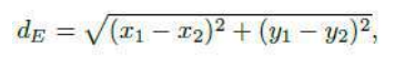

其中 (x1,y1) 是我家在某个坐标系中的位置(比如使用 GPS 追踪器),(x2,y2) 是商店的位置。
如果我告诉你我的城镇是按网格街区系统布局的,这在汽车发明和创新城镇规划者发明之间建造的城镇中很常见,那么你可能会使用不同的度量。你会测量我家和商店之间在“南北”方向上的距离,以及在“东西”方向上的距离,然后将这两个距离相加。这对应于我实际需要步行的距离。它通常被称为城市街区距离(city-block distance)或曼哈顿距离(Manhattan distance),看起来像这样:
![]()
这次讨论的目的是为了表明衡量距离的方式不止一种,而且它们可以提供截然不同的答案。这两种不同的距离可以在图 11 中看到。在数学上,这些距离度量被称为度量(metrics)。一个度量函数或范数接受两个输入并返回一个标量(距离),该标量必须是正数,并且当且仅当两个点相同时才为 0,对称的(即到商店的距离与返回的距离相同),并且遵守三角不等式,即从 a 到 b 的距离加上从 b 到 c 的距离不应小于从 a 到 c 的直接距离。
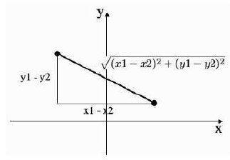
图 10:两点之间的欧几里得距离和城市街区距离。
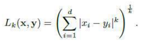
我们不得不分析的大多数数据都存在于远超两个维度。幸运的是,我们所了解的欧几里得距离可以很好地推广到更高维度(城市街区度量也一样)。事实上,这两种度量都是一类可在任意维度中工作的度量的实例。通用的度量是闵可夫斯基距离(Minkowski metric),它写为:
如果我们设置 ,我们就得到了城市街区距离(方程 (7.12)),而 则得到欧几里得距离(方程 (7.11))。因此,你可能会看到欧几里得度量被写为 L2 范数,城市街区距离被写为 L1 范数。这些范数还有另一个有趣的特性。回想一下,我们可以定义一组数字的不同平均值。如果我们将平均值定义为最小化到每个数据点距离之和的点,那么结果是均值(mean)最小化欧几里得距离(平方和距离),而中位数(median)最小化 L1 度量。
根据数据空间的不同,还有许多其他可能的度量可供选择。我们通常假设空间是平坦的(如果不是,那么这些技术都不起作用,我们也不想担心这个问题)。然而,查看其他度量仍然可能是有益的。假设我们希望我们的分类器能够识别图像,例如人脸。我们拍摄一组人脸的数字照片,并使用像素值作为特征。然后我们使用我们刚刚看到的最近邻算法来识别每个人脸。即使我们确保所有照片都是完全正面拍摄的,仍然有一些事情会妨碍这种方法。一个是头部(或相机)角度的微小变化可能会产生影响;另一个是人脸与相机之间不同的距离(缩放)会改变结果;还有一个是不同的照明条件会产生影响。我们可以尝试在预处理中修复所有这些问题,但还有另一种选择:使用对这些变化不变的不同度量,即,它不会随着这些变化而变化。不变度量的思想是找到那些忽略你不希望发生的变化的度量。因此,如果你希望能够旋转形状并仍然识别它们,你需要一个对旋转不变的度量。
图像中常用的一种不变度量是切线距离(tangent distance),它是一阶导数泰勒展开式的近似值,对于小幅旋转和缩放效果非常好;例如,它曾用于将一组手写字母的最近邻分类的最终错误率减半。不变度量是一个有趣的深入研究话题,如果你感兴趣,可以在“进一步阅读”部分找到它们的参考文献。
We have computed the distance between points as the Euclidean distance, which is something
that you learnt about in high school. However, it is not the only option, nor is it necessarily the most
useful. In this section we will look at the underlying idea behind distance calculations and possible
alternatives.
If I were to ask you to find the distance between my house and the nearest shop, then your first
guess might involve taking a map of my town, locating my house and the shop, and using a ruler to
measure the distance between them. By careful application of the map scale you can now tell me how
far it is. However, when I set out to buy some milk I’m liable to find that I have to walk rather further
than you’ve told me, since the direct line that you measured would involve walking through (or over)
several houses, and some serious fence-scaling. Your ‘as the crow flies’ distance is the shortest possible
path, and it is the straight-line, or Euclidean, distance. You can measure it on the map by just using a
ruler, but it essentially consists of measuring the distance in one direction (we’ll call it
north-south) and then the distance in another direction that is perpendicular to the first (let’s call it
east-west) and then squaring them, adding them together, and then taking the square root of that.
Writing that out, the Euclidean distance that we are all used to is:
where (x1, y1) is the location of my house in some coordinate system (say by using a GPS tracker) and
(x2, y2) is the location of the shop.
If I told you that my town was laid out on a grid block system, as is common in towns that were
built in the interval between the invention of the motor car and the invention of innovative town
planners, then you would probably use a different measure. You would measure the distance between
my house and the shop in the ‘north-south’ direction and the distance in the ‘east-west’ direction, and
then add the two distances together. This would correspond to the distance I actually had to walk. It is
often known as the city-block or Manhattan distance and looks like:
The point of this discussion is to show that there is more than one way to measure a distance,
and that they can provide radically different answers. These two different distances can be seen in
Figure 11. Mathematically, these distance measures are known as metrics. A metric function or norm
takes two inputs and gives a scalar (the distance) back, which is positive, and 0 if and only if the two
points are the same, symmetric (so that the distance
to the shop is the same as the distance back), and obeys the triangle inequality, which says that the
distance from a to b plus the distance from b to c should not be less than the direct distance from a to FIGURE 10: The Euclidean and city-block distances between two points.
Most of the data that we are going to have to analyse lives in rather more than two dimensions.
Fortunately, the Euclidean distance that we know about generalises very well to higher dimensions (and
so does the city-block metric). In fact, these two measures are both instances of a class of metrics that
work in any number of dimensions. The general measure is the Minkowski metric and it is written as:
If we put k = 1 then we get the city-block distance (Equation (7.12)), and k = 2 gives the
Euclidean distance (Equation (7.11)). Thus, you might possibly see the Euclidean metric written as the L2
norm and the city-block distance as the L1 norm. These norms have another interesting feature.
Remember that we can define different averages of a set of numbers. If we define the average as the
point that minimises the sum of the distance to every datapoint, then it turns out that the mean
minimises the Euclidean distance (the sum-of-squares distance), and the median minimises the L1
metric.
There are plenty of other possible metrics to choose, depending upon the dataspace. We
generally assume that the space is flat (if it isn’t, then none of these techniques work, and we don’t
want to worry about that). However, it can still be beneficial to look at other metrics. Suppose that we
want our classifier to be able to recognise images, for example of faces. We take a set of digital photos
of faces and use the pixel values as features. Then we use the nearest neighbour algorithm that we’ve
just seen to identify each face. Even if we ensure that all of the photos are taken fully face-on, there are
still a few things that will get in the way of this method. One is that slight variations in the angle of the
head (or the camera) could make a difference; another is that different distances between the face and
the camera (scaling) will change the results; and another is that different lighting conditions will make a
difference. We can try to fix all of these things in preprocessing, but there is also another alternative:
use a different metric that is invariant to these changes, i.e., it does not vary as they do. The idea of
invariant metrics is to find measures that ignore changes that you don’t want. So if you want to be able
to rotate shapes around and still recognize them, you need a metric that is invariant to rotation.
A common invariant metric in use for images is the tangent distance, which is an approximation
to the Taylor expansion in first derivatives, and works very well for small rotations and scalings; for
example, it was used to halve the final error rate on nearest neighbor classification of a set of
handwritten letters. Invariant metrics are an interesting topic for further study, and there is a reference
for them in the Further Reading section if you are interested.