机器学习
遗传算法(GAs)旨在搜索候选假设空间以识别最佳假设。在遗传算法中,“最佳假设”被定义为优化了手头问题预定义数值度量的那个,这个度量被称为假设适应度。例如,如果学习任务是根据输入和输出的训练样本来逼近一个未知函数,那么适应度可以定义为该假设在这些训练数据上的准确性。如果任务是学习下棋的策略,那么适应度可以定义为个体在与当前种群中其他个体对弈时赢得的局数。
虽然遗传算法的不同实现方式在细节上有所不同,但它们通常具有以下结构:算法通过迭代更新一个被称为“种群”的假设池来运行。在每次迭代中,种群的所有成员都根据适应度函数进行评估。然后,通过概率性地从当前种群中选择适应度高的个体来生成新种群。这些被选择的个体中有一部分会完整地进入下一代种群。其他个体则被用作基础,通过应用**交叉(crossover)和变异(mutation)**等遗传操作来创建新的子代个体。
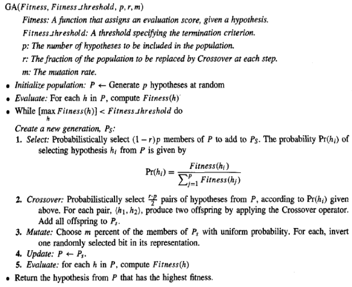
该算法的输入包括用于对候选假设进行排序的适应度函数、定义终止算法可接受适应度水平的阈值、要维护的种群大小,以及确定如何生成后续种群的参数:每代要替换的种群比例和变异率。
请注意,在此算法中,主循环的每次迭代都会根据当前种群产生新一代的假设。首先,从当前种群中选择一定数量的假设纳入下一代。这些选择是概率性的,选择假设 hi 的概率由以下公式给出:
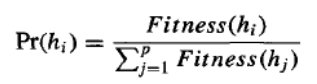
因此,一个假设被选择的概率与其自身的适应度成正比,并与当前种群中其他竞争假设的适应度成反比。
一旦当前代中的这些成员被选中纳入下一代种群,就会使用交叉操作生成额外的成员。交叉,在下一节将详细定义,它从当前代中选取两个父代假设,通过重组两个父代的部分来创建两个子代假设。父代假设是根据方程 (9.1) 给出的概率函数,从当前种群中概率性地选择的。在通过此交叉操作创建新成员后,新一代种群现在包含所需的成员数量。此时,这些成员中的一定比例 m 会被随机选择,并进行随机变异以改变这些成员。
因此,这个遗传算法通过随机化、并行束搜索来寻找根据适应度函数表现良好的假设。在以下小节中,我们将更详细地描述该算法中使用的假设表示和遗传操作符。
表示假设
遗传算法中的假设通常由位串表示,这样它们可以通过变异和交叉等遗传操作符轻松操作。这些位串表示的假设可以非常复杂。例如,if-then 规则集可以通过选择一种规则编码方式轻松表示,该方式为每个规则前置条件和后置条件分配特定的子串。
为了了解 if-then 规则如何通过位串编码,首先考虑我们如何使用位串来描述单个属性值的约束。举个例子,考虑属性 Outlook,它可以取 Sunny、Overcast 或 Rain 三个值。表示 Outlook 约束的一种明显方法是使用长度为三的位串,其中每个位位置对应其三个可能值中的一个。在某个位置放置 1 表示允许该属性取相应的值。例如,字符串 010 表示 Outlook 必须取这些值中的第二个,即 Outlook = Overcast。类似地,字符串 011 表示更通用的约束,允许两个可能的值,即 (Outlook = Overcast ∨ Rain)。注意 111 表示最通用的可能约束,表示我们不关心该属性取其哪个可能值。
鉴于这种表示单个属性约束的方法,多个属性约束的合取可以很容易地通过连接相应的位串来表示。例如,考虑第二个属性 Wind,它可以取 Strong 或 Weak 值。一个规则前置条件,例如:
(Outlook = Overcast ∧ Rain) ∧ (Wind = Strong)
可以用以下长度为五的位串表示:
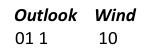
规则后置条件(例如 PlayTennis = yes)可以用类似的方式表示。因此,整个规则可以通过连接描述规则前置条件的位串以及描述规则后置条件的位串来描述。例如,规则:
IF Wind = Strong THEN PlayTennis = yes
将由以下字符串表示:
![]()
其中前三位描述了 Outlook 上的“不关心”约束,接下来的两位描述了 Wind 上的约束,最后两位描述了规则后置条件(这里我们假设 PlayTennis 可以取 Yes 或 No 值)。请注意,表示规则的位串包含假设空间中每个属性的子串,即使该属性不受规则前置条件的约束。这会产生一个固定长度的位串表示规则,其中特定位置的子串描述了特定属性的约束。鉴于这种单个规则的表示,我们可以通过类似地连接单个规则的位串表示来表示规则集。
在设计用于某个假设空间的位串编码时,有必要确保每个语法上合法的位串都表示一个定义明确的假设。举例说明,请注意在上一段的规则编码中,位串 111 10 11 表示一个后置条件不约束目标属性 PlayTennis 的规则。如果我们希望避免考虑这种假设,我们可以采用不同的编码(例如,只为 PlayTennis 后置条件分配一位来表示值是 Yes 还是 No),改变遗传操作符使其明确避免构造此类位串,或者简单地为此类位串分配非常低的适应度。
在某些遗传算法中,假设用符号描述而不是位串表示。
遗传操作符
遗传算法中后代的生成由一组操作符决定,这些操作符重组并变异当前种群中选定的成员。这些操作符对应于生物进化中发现的遗传操作的理想化版本。最常见的两种操作符是交叉和变异。
交叉操作符通过复制每个父代的选定位来从两个父代字符串产生两个新的子代。每个子代中位置 i 的位是从两个父代中一个父代中位置 i 的位复制的。选择哪个父代贡献位置 i 的位由一个额外的字符串(称为交叉掩码)决定。为了说明这一点,考虑表顶部所示的单点交叉操作符。考虑在这种情况下两个子代中靠上的那个。这个子代的前五位来自第一个父代,其余六位来自第二个父代,因为交叉掩码 11111000000 指定了每个位位置的这些选择。第二个子代使用相同的交叉掩码,但交换了两个父代的角色。因此,它包含第一个子代未使用的位。在单点交叉中,交叉掩码总是这样构造:它以一个包含 n 个连续 1 的字符串开始,然后是完成字符串所需的 0 的数量。这导致子代中前 n 个位由一个父代贡献,其余位由第二个父代贡献。每次应用单点交叉操作符时,交叉点 n 都是随机选择的,然后创建并应用交叉掩码。
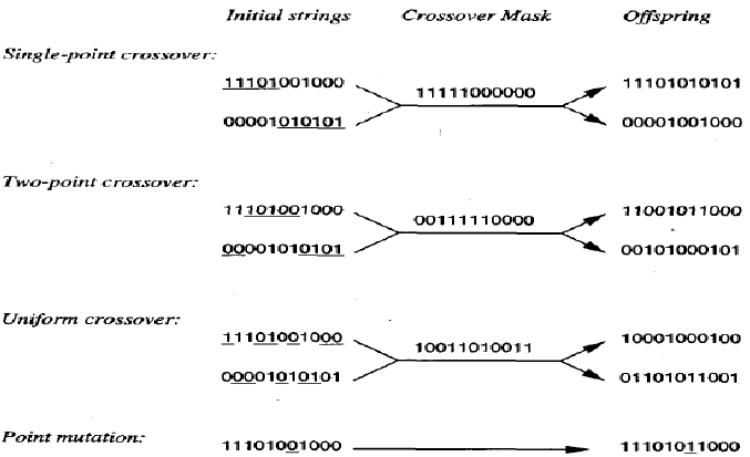
在两点交叉中,子代是通过将一个父代的中间片段替换到第二个父代字符串的中间来创建的。换句话说,交叉掩码是一个以若干个 0 开头(可能为 0 个),接着是 n1 个连续 1 的字符串,然后是完成字符串所需的 0 的数量的字符串。每次应用两点交叉操作符时,通过随机选择整数 n0 和 n1 来生成掩码。
适应度函数和选择
适应度函数定义了对潜在假设进行排序并概率性地选择它们以纳入下一代种群的标准。如果任务是学习分类规则,那么适应度函数通常包含一个组件,用于评估规则在一组提供的训练样本上的分类准确性。通常也可以包含其他标准,例如规则的复杂性或泛化性。更一般地,当位串假设被解释为一个复杂过程时(例如,当位串表示一系列将被链接起来以控制机器人设备的 if-then 规则时),适应度函数可以衡量所得过程的整体性能,而不是单个规则的性能。
在我们原型遗传算法中,如上表所示,假设被选择的概率由其适应度与当前种群中其他成员适应度的比率给出,如上述方程所示。这种方法有时被称为适应度比例选择,或轮盘赌选择。
还提出了其他使用适应度选择假设的方法。例如,在锦标赛选择中,首先从当前种群中随机选择两个假设。以某个预定义概率 p 选择这两个中适应度更高的那个,并以概率 选择适应度更低的假设。锦标赛选择通常比适应度比例选择产生更多样化的种群。在另一种称为排名选择的方法中,当前种群中的假设首先按适应度排序。然后,假设被选择的概率与它在此排序列表中的排名成正比,而不是与它的适应度成正比。
The problem addressed by GAS is to search a space of candidate hypotheses to identify the best
hypothesis. In GAS the "best hypothesis" is defined as the one that optimizes a predefined numerical
measure for the problem at hand, called b the hypothesis fitness. For example, if the learning task is the
problem of approximating an unknown function given training examples of its input and output, then
fitness could be defined as the accuracy of the hypothesis over this training data. If the task is to learn a
strategy for playing chess, fitness could be defined as the number of games won by the individual when
playing against other individuals in the current population.
Although different implementations of genetic algorithms vary in their details, they typically share the
following structure: The algorithm operates by iteratively updating a pool of hypotheses, called the
population. On each iteration, all members of the population are evaluated according to the fitness
function. A new population is then generated by probabilistically selecting the fit individuals from the
current population. Some of these selected individuals are carried forward into the next generation
population intact. Others are used as the basis for creating new offspring individuals by applying genetic
operations such as crossover and mutation.
The inputs to this algorithm include the fitness function for ranking candidate hypotheses, a
threshold defining an acceptable level of fitness for terminating the algorithm, the size of the
population to be maintained, and parameters that determine how successor populations are to be
generated: the fraction of the population to be replaced at each generation and the mutation rate.
Notice in this algorithm each iteration through the main loop produces a new generation of hypotheses
based on the current population. First, a certain number of hypotheses from the current population are
selected for inclusion in the next generation. These are selected probabilistically, where the probability
of selecting hypothesis hi is given by
Thus, the probability that a hypothesis will be selected is proportional to its own fitness and is
inversely proportional to the fitness of the other competing hypotheses in the current population.
Once these members of the current generation have been selected for inclusion in the next generation
population, additional members are generated using a crossover operation. Crossover, defined in detail
in the next section, takes two parent hypotheses from the current generation and creates two offspring
hypotheses
by recombining portions of both parents. The parent hypotheses are chosen probabilistically from the
current population, again using the probability function given by Equation (9.1). After new members
have been created by this crossover operation, the new generation population now contains the
101
desired number of members. At this point, a certain fraction m of these members are chosen at
random, and random mutations all performed to alter these members.
This GA algorithm thus performs a randomized, parallel beam search for hypotheses that perform well
according to the fitness function. In the following subsections, we describe in more detail the
representation of hypotheses and genetic operators used in this algorithm.
Representing Hypotheses
Hypotheses in GAS are often represented by bit strings, so that they can be easily manipulated
by genetic operators such as mutation and crossover. The hypotheses represented by these bit strings
can be quite complex. For example, sets of if-then rules can easily be represented in this way, by
choosing an encoding of rules that allocates specific substrings for each rule precondition and
postcondition.
To see how if-then rules can be encoded by bit strings, .first consider how we might use a bit
string to describe a constraint on the value of a single attribute. To pick an example, consider the
attribute Outlook, which can take on any of the three values Sunny, Overcast, or Rain. One obvious way
to represent a constraint on Outlook is to use a bit string of length three, in which each bit position
corresponds to one of its three possible values. Placing a 1 in some position indicates that the attribute
is allowed to take on the corresponding value. For example, the string 010 represents the constraint
that Outlook must take on the second of these values, or Outlook = Overcast. Similarly, the string 011
represents the more general constraint that allows two possible values, or (Outlook = Overcast v Rain).
Note 11 1 represents the most general possible constraint, indicating that we don't care which of its
possible values the attribute takes on.
Given this method for representing constraints on a single attribute, conjunctions of constraints
on multiple attributes can easily be represented by concatenating the corresponding bit strings. For
example, consider a second attribute, Wind, that can take on the value Strong or Weak. A rule
precondition such as
(Outlook = Overcast ^Rain) A (Wind = Strong)
can then be represented by the following bit string of length five:
Outlook Wind
01 1
10
Rule postconditions (such as PlayTennis = yes) can be represented in a similar fashion. Thus, an entire
rule can be described by concatenating the bit strings describing the rule preconditions, together with
the bit string describing the rule postcondition. For example, the rule
IF Wind = Strong THEN PlayTennis = yes
would be represented by the string
Outlook Wind PlayTennis
111
10
10
where the first three bits describe the "don't care" constraint on Outlook, the next two bits describe the
constraint on Wind, and the final two bits describe the rule postcondition (here we assume PlayTennis
102
can take on the values Yes or No). Note the bit string representing the rule contains a substring for each
attribute in the hypothesis space, even if that attribute is not constrained by the rule preconditions. This
yields a fixed length bit-string representation for rules, in which substrings at specific locations describe
constraints on specific attributes. Given this representation for single rules, we can represent sets of
rules by similarly concatenating the bit string representations of the individual rules.
In designing a bit string encoding for some hypothesis space, it is useful to arrange for every
syntactically legal bit string to represent a well-defined hypothesis. To illustrate, note in the rule
encoding in the above paragraph the bit string 11 1 10 11 represents a rule whose postcondition does
not constrain the target attribute PlayTennis. If we wish to avoid considering this hypothesis, we may
employ a different encoding (e.g., allocate just one bit to the PlayTennis postcondition to indicate
whether the value is Yes or No), alter the genetic operators so that they explicitly avoid constructing
such bit strings, or simply assign a very low fitness to such bit strings.
In some GAS, hypotheses are represented by symbolic descriptions rather than bit strings.
Genetic Operators
The generation of successors in a GA is determined by a set of operators that recombine and
mutate selected members of the current population. These operators correspond to idealized versions
of the genetic operations found in biological evolution. The two most common operators are crossover
and mutation.
The crossover operator produces two new offspring from two parent strings, by copying
selected bits from each parent. The bit at position i in each offspring is copied from the bit at position i
in one of the two parents. The choice of which parent contributes the bit for position i is determined by
an additional string called the crossover mask. To illustrate, consider the single-point crossover
operator at the top of Table Consider the topmost of the two offspring in this case. This offspring takes
its first five bits from the first parent and its remaining six bits from the second parent, because the
crossover mask 11 11 1000000 specifies these choices for each of the bit positions. The second offspring
uses the same crossover mask, but switches the roles of the two parents. Therefore, it contains the bits
that were not used by the first offspring. In single-point crossover, the crossover mask is always
constructed so that it begins with a string containing n contiguous Is, followed by the necessary number
of 0s to complete the string. This results in offspring in which the first n bits are contributed by one
parent and the remaining bits by the second parent. Each time the single-point crossover operator is
applied the crossover point n is chosen at random, and the crossover mask is then created and applied.
103
In two-point crossover, offspring are created by substituting intermediate segments of one parent into
the middle of the second parent string. Put another way, the crossover mask is a string beginning with
no zeros, followed by a contiguous string of nl ones, followed by the necessary number of zeros to
complete the string. Each time the two-point crossover operator is applied, a mask is generated by
randomly choosing the integers no and nl.
Fitness Function and Selection
The fitness function defines the criterion for ranking potential hypotheses and for
probabilistically selecting them for inclusion in the next generation population. If the task is to learn
classification rules, then the fitness function typically has a component that scores the classification
accuracy of the rule over a set of provided training examples. Often other criteria may be included as
well, such as the complexity or generality of the rule. More generally, when the bit-string hypothesis is
interpreted as a complex procedure (e.g., when the bit string represents a collection of if-then rules that
will be chained together to control a robotic device), the fitness function may measure the overall
performance of the resulting procedure rather than performance of individual rules.
In our prototypical GA shown in above Table , the probability that a hypothesis will be selected is given
by the ratio of its fitness to the fitness of other members of the current population as seen in Equation
above . This method is sometimes called fitness proportionate selection, or roulette wheel selection.
Other methods for using fitness to select hypotheses have also been proposed. For example, in
tournament selection, two hypotheses are first chosen at random from the current population. With
some predefined probability p the more fit of these two is then selected, and with probability (1 - p) the
less fit hypothesis is selected. Tournament selection often yields a more diverse population than fitness
proportionate selection. In another method called rank selection, the hypotheses in the current
population are first sorted by fitness. The probability that a hypothesis will be selected is then
proportional to its rank in this sorted list, rather than its fitness.