Python 机器学习
朴素贝叶斯算法简介
朴素贝叶斯算法是一种分类技术,基于应用贝叶斯定理,并有一个强烈的假设:所有预测变量相互独立。简单来说,这个假设是:一个特征在一个类别中的存在与同一类别中任何其他特征的存在是独立的。例如,如果一部手机有触摸屏、互联网功能、好摄像头等,它可能被认为是智能手机。尽管所有这些特征都相互依赖,但它们独立地对该手机是智能手机的概率做出贡献。
在贝叶斯分类中,主要兴趣在于找到后验概率,即在给定某些观察到的特征的情况下,标签的概率 P(L∣textfeatures)。借助贝叶斯定理,我们可以将其表示为定量形式,如下所示:
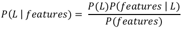
这里,P(L∣textfeatures) 是类别的后验概率。
P(L) 是类别的先验概率。
P(textfeatures∣L) 是似然,即给定类别的预测变量的概率。
P(textfeatures) 是预测变量的先验概率。
使用 Python 中的朴素贝叶斯构建模型
Python 库 Scikit-learn 是最有用的库,可帮助我们在 Python 中构建朴素贝叶斯模型。在 Scikit-learn Python 库下,我们有以下三种类型的朴素贝叶斯模型:
高斯朴素贝叶斯 (Gaussian Naïve Bayes)
这是最简单的朴素贝叶斯分类器,其假设是每个标签的数据都来自一个简单的高斯分布。
多项式朴素贝叶斯 (Multinomial Naïve Bayes)
另一种有用的朴素贝叶斯分类器是多项式朴素贝叶斯,其中假设特征来自简单的多项式分布。这种朴素贝叶斯最适合表示离散计数的特征。
伯努利朴素贝叶斯 (Bernoulli Naïve Bayes)
另一个重要的模型是伯努利朴素贝叶斯,其中特征被假定为二元的(0 和 1)。使用“词袋”模型的文本分类可以是伯努利朴素贝叶斯的一个应用。
示例
根据我们的数据集,我们可以选择上面解释的任何一种朴素贝叶斯模型。在这里,我们将在 Python 中实现高斯朴素贝叶斯模型:
我们将从所需的导入开始,如下所示:
import numpy as np
import matplotlib.pyplot as plt
import seaborn as sns; sns.set()
现在,通过使用 Scikit-learn 的 make_blobs() 函数,我们可以生成具有高斯分布的点簇,如下所示:
from sklearn.datasets import make_blobs
X, y = make_blobs(300, 2, centers=2, random_state=2, cluster_std=1.5)
plt.scatter(X[:, 0], X[:, 1], c=y, s=50, cmap='summer');
plt.show() # 添加这一行以显示图形
(此处应插入一个散点图,显示两类高斯分布的点簇)
接下来,为了使用 GaussianNB 模型,我们需要导入并创建其对象,如下所示:
from sklearn.naive_bayes import GaussianNB
model_GNB = GaussianNB() # 修正变量名,保持一致性
model_GNB.fit(X, y);
现在,我们必须进行预测。这可以在生成一些新数据后完成,如下所示:
rng = np.random.RandomState(0)
Xnew = [-6, -14] + [14, 18] * rng.rand(2000, 2)
ynew = model_GNB.predict(Xnew)
接下来,我们绘制新数据以找到其边界:
plt.scatter(X[:, 0], X[:, 1], c=y, s=50, cmap='summer')
lim = plt.axis()
plt.scatter(Xnew[:, 0], Xnew[:, 1], c=ynew, s=20, cmap='summer', alpha=0.1)
plt.axis(lim);
plt.show() # 添加这一行以显示图形
(此处应插入一个散点图,显示原始数据和预测新数据的边界)
现在,借助以下代码行,我们可以找到第一个和第二个标签的后验概率:
yprob = model_GNB.predict_proba(Xnew)
print(yprob[-10:].round(3))
输出
[[0.998 0.002]
 [1.    0.   ]
 [0.987 0.013]
 [1.    0.   ]
 [1.    0.   ]
 [1.    0.   ]
 [1.    0.   ]
 [1.    0.   ]
 [0.    1.   ]
 [0.986 0.014]]
优缺点 (Pros & Cons)
优点 (Pros)
以下是使用朴素贝叶斯分类器的一些优点:
- 朴素贝叶斯分类实现简单且速度快。
- 它比逻辑回归等判别模型收敛更快。
- 它需要较少的训练数据。
- 它本质上具有高度可扩展性,或者它们与预测变量和数据点的数量呈线性关系。
- 它可以进行概率预测,并且可以处理连续和离散数据。
- 朴素贝叶斯分类算法可用于二元和多类别分类问题。
缺点 (Cons)
以下是使用朴素贝叶斯分类器的一些缺点:
- 朴素贝叶斯分类最重要的缺点之一是其强大的特征独立性,因为在现实生活中,几乎不可能拥有一组完全相互独立的特征。
- 朴素贝叶斯分类的另一个问题是其“零频率”,这意味着如果一个分类变量有一个类别但在训练数据集中未被观察到,那么朴素贝叶斯模型将为其分配零概率,并且将无法进行预测。
朴素贝叶斯分类的应用 (Applications of Naïve Bayes classification)
以下是朴素贝叶斯分类的一些常见应用:
- 实时预测:由于其易于实现和快速计算,它可用于实时进行预测。
- 多类别预测:朴素贝叶斯分类算法可用于预测目标变量多个类别的后验概率。
- 文本分类:由于多类别预测的特点,朴素贝叶斯分类算法非常适合文本分类。这就是为什么它也用于解决垃圾邮件过滤和情感分析等问题。
- 推荐系统:除了协同过滤等算法,朴素贝叶斯构建了一个推荐系统,可用于过滤未见信息并预测用户是否会喜欢给定的资源。
13. Classification Algorithms Machine
- Naïve
Learning Bayes
with Python
Introduction to Naïve Bayes Algorithm
Naïve Bayes algorithms is a classification technique based on applying Bayes’ theorem
with a strong assumption that all the predictors are independent to each other. In simple
words, the assumption is that the presence of a feature in a class is independent to the
presence of any other feature in the same class. For example, a phone may be considered
as smart if it is having touch screen, internet facility, good camera etc. Though all these
features are dependent on each other, they contribute independently to the probability of
that the phone is a smart phone.
In Bayesian classification, the main interest is to find the posterior probabilities i.e. the
probability of a label given some observed features, P(L | features). With the help of Bayes
theorem, we can express this in quantitative form as follows:
P(L)P(features | L)
P(L | features) =
P(features)
Here, P(L | features) is the posterior probability of class.
P(L) is the prior probability of class.
P(features | L) is the likelihood which is the probability of predictor given class.
P(features) is the prior probability of predictor.
Building model using Naïve Bayes in Python
Python library, Scikit learn is the most useful library that helps us to build a Naïve Bayes
model in Python. We have the following three types of Naïve Bayes model under Scikit
learn Python library:
Gaussian Naïve Bayes
It is the simplest Naïve Bayes classifier having the assumption that the data from each
label is drawn from a simple Gaussian distribution.
Multinomial Naïve Bayes
Another useful Naïve Bayes classifier is Multinomial Naïve Bayes in which the features are
assumed to be drawn from a simple Multinomial distribution. Such kind of Naïve Bayes are
most appropriate for the features that represents discrete counts.
Bernoulli Naïve Bayes
Another important model is Bernoulli Naïve Bayes in which features are assumed to be
binary (0s and 1s). Text classification with ‘bag of words’ model can be an application of
Bernoulli Naïve Bayes.
86
Machine Learning with Python
Example
Depending on our data set, we can choose any of the Naïve Bayes model explained above.
Here, we are implementing Gaussian Naïve Bayes model in Python:
We will start with required imports as follows:
import numpy as np
import matplotlib.pyplot as plt
import seaborn as sns; sns.set()
Now, by using make_blobs() function of Scikit learn, we can generate blobs of points
with Gaussian distribution as follows:
from sklearn.datasets import make_blobs
X, y = make_blobs(300, 2, centers=2, random_state=2, cluster_std=1.5)
plt.scatter(X[:, 0], X[:, 1], c=y, s=50, cmap='summer');
Next, for using GaussianNB model, we need to import and make its object as follows:
from sklearn.naive_bayes import GaussianNB
model_GBN = GaussianNB()
model_GNB.fit(X, y);
Now, we have to do prediction. It can be done after generating some new data as follows:
rng = np.random.RandomState(0)
Xnew = [-6, -14] + [14, 18] * rng.rand(2000, 2)
ynew = model_GNB.predict(Xnew)
Next, we are plotting new data to find its boundaries:
plt.scatter(X[:, 0], X[:, 1], c=y, s=50, cmap='summer')
lim = plt.axis()
plt.scatter(Xnew[:, 0], Xnew[:, 1], c=ynew, s=20, cmap='summer', alpha=0.1)
plt.axis(lim);
Now, with the help of following line of codes, we can find the posterior probabilities of first
and second label:
yprob = model_GNB.predict_proba(Xnew)
yprob[-10:].round(3)
87
Machine Learning with Python
Output
array([[0.998, 0.002],
[1.
, 0.
],
[0.987, 0.013],
[1.
, 0.
],
[1.
, 0.
],
[1.
, 0.
],
[1.
, 0.
],
[1.
, 0.
],
[0.
, 1.
],
[0.986, 0.014]])
Pros & Cons
Pros
The followings are some pros of using Naïve Bayes classifiers:
Naïve Bayes classification is easy to implement and fast.
It will converge faster than discriminative models like logistic regression.
It requires less training data.
It is highly scalable in nature, or they scale linearly with the number of predictors
and data points.
It can make probabilistic predictions and can handle continuous as well as discrete
data.
Naïve Bayes classification algorithm can be used for binary as well as multi-class
classification problems both.
Cons
The followings are some cons of using Naïve Bayes classifiers:
One of the most important cons of Naïve Bayes classification is its strong feature
independence because in real life it is almost impossible to have a set of features
which are completely independent of each other.
Another issue with Naïve Bayes classification is its ‘zero frequency’ which means
that if a categorial variable has a category but not being observed in training data
set, then Naïve Bayes model will assign a zero probability to it and it will be unable
to make a prediction.
88
Machine Learning with Python
Applications of Naïve Bayes classification
The following are some common applications of Naïve Bayes classification:
Real-time prediction: Due to its ease of implementation and fast computation, it can be
used to do prediction in real-time.
Multi-class prediction: Naïve Bayes classification algorithm can be used to predict
posterior probability of multiple classes of target variable.
Text classification: Due to the feature of multi-class prediction, Naïve Bayes
classification algorithms are well suited for text classification. That is why it is also used
to solve problems like spam-filtering and sentiment analysis.
Recommendation system: Along with the algorithms like collaborative filtering, Naïve
Bayes makes a Recommendation system which can be used to filter unseen information
and to predict weather a user would like the given resource or not.