Python 机器学习
我们可以使用各种指标来评估机器学习算法的性能,包括分类算法和回归算法。我们必须仔细选择评估机器学习性能的指标,因为:
- 机器学习算法的性能如何衡量和比较将完全取决于您选择的指标。
- 您如何衡量结果中各种特征的重要性将完全受您选择的指标的影响。
分类问题的性能指标
我们已经在前面的章节中讨论了分类及其算法。在这里,我们将讨论可用于评估分类问题预测的各种性能指标。
混淆矩阵 (Confusion Matrix)
这是衡量分类问题性能最简单的方法,其中输出可以是两种或更多种类型的类别。混淆矩阵只不过是一个具有两个维度(即“实际”和“预测”)的表格,而且,这两个维度都有“真阳性 (TP)”、“真阴性 (TN)”、“假阳性 (FP)”、 “假阴性 (FN)”如下所示:
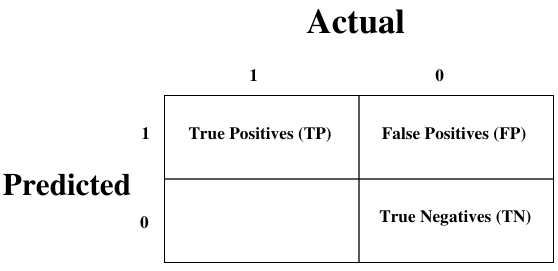
与混淆矩阵相关的术语解释如下:
- 真阳性 (TP):当数据点的实际类别和预测类别均为 1 时。
- 真阴性 (TN):当数据点的实际类别和预测类别均为 0 时。
- 假阳性 (FP):当数据点的实际类别为 0 且预测类别为 1 时。
- 假阴性 (FN):当数据点的实际类别为 1 且预测类别为 0 时。
我们可以使用 sklearn.metrics 中的 confusion_matrix 函数来计算我们分类模型的混淆矩阵。
分类准确率 (Classification Accuracy)
它是分类算法最常见的性能指标。它可以定义为正确预测的数量与所有预测数量的比率。我们可以使用混淆矩阵通过以下公式轻松计算:
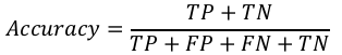
我们可以使用 sklearn.metrics 中的 accuracy_score 函数来计算我们分类模型的准确率。
分类报告 (Classification Report)
此报告包含精确率、召回率、F1 分数和支持度的分数。它们解释如下:
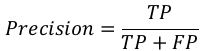
精确率 (Precision)
精确率,用于文档检索,可以定义为我们的机器学习模型返回的正确文档的数量。我们可以使用混淆矩阵通过以下公式轻松计算:
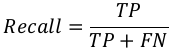
召回率或敏感度 (Recall or Sensitivity)
召回率可以定义为我们的机器学习模型返回的阳性数量。我们可以使用混淆矩阵通过以下公式轻松计算:
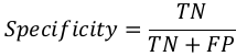
特异性 (Specificity)
特异性,与召回率相反,可以定义为我们的机器学习模型返回的阴性数量。我们可以使用混淆矩阵通过以下公式轻松计算:
支持度 (Support)
支持度可以定义为每个目标值类别中真实响应的样本数量。
F1 分数 (F1 Score)
此分数将给出精确率和召回率的调和平均值。数学上,F1 分数是精确率和召回率的加权平均值。F1 的最佳值为 1,最差值为 0。我们可以使用以下公式计算 F1 分数:
F1 = 2 ∗ (precision ∗ recall) / (precision + recall) #F1=2∗(精确率+召回率)(精确率∗召回率)
F1 分数在精确率和召回率方面具有相等的相对贡献。
我们可以使用 sklearn.metrics 中的 classification_report 函数来获取我们分类模型的分类报告。
AUC(ROC 曲线下面积)(AUC (Area Under ROC curve))
AUC (Area Under Curve)-ROC (Receiver Operating Characteristic) 是一个性能指标,基于变化的阈值,用于分类问题。顾名思义,ROC 是一条概率曲线,AUC 衡量可分离性。简单来说,AUC-ROC 指标将告诉我们模型区分类别的能力。AUC 越高,模型越好。
数学上,它可以通过绘制 TPR(真阳性率,即敏感度或召回率)与 FPR(假阳性率,即 1-特异性)在各种阈值下创建。下图显示了 ROC,AUC 的 Y 轴为 TPR,X 轴为 FPR:
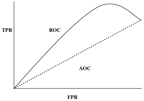
我们可以使用 sklearn.metrics 中的 roc_auc_score 函数来计算 AUC-ROC。
LOGLOSS(对数损失)(LOGLOSS (Logarithmic Loss))
它也称为逻辑回归损失或交叉熵损失。它基本上定义在概率估计上,并衡量分类模型的性能,其中输入是介于 0 和 1 之间的概率值。通过将其与准确率区分开来可以更清楚地理解它。我们知道准确率是我们模型中预测(预测值 = 实际值)的计数,而对数损失是根据预测与实际标签的差异程度来衡量预测的不确定性量。借助对数损失值,我们可以更准确地了解模型的性能。我们可以使用 sklearn.metrics 中的 log_loss 函数来计算对数损失。
示例 (Example)
以下是一个简单的 Python 示例,它将向我们展示如何在二元分类模型上使用上面解释的性能指标:
from sklearn.metrics import confusion_matrix
from sklearn.metrics import accuracy_score
from sklearn.metrics import classification_report
from sklearn.metrics import roc_auc_score
from sklearn.metrics import log_loss

X_actual = [1, 1, 0, 1, 0, 0, 1, 0, 0, 0]
Y_predic = [1, 0, 1, 1, 1, 0, 1, 1, 0, 0]

results = confusion_matrix(X_actual, Y_predic)
print ('Confusion Matrix :')
print(results)

print ('Accuracy Score is',accuracy_score(X_actual, Y_predic))

print ('Classification Report : ')
print (classification_report(X_actual, Y_predic))

print('AUC-ROC:',roc_auc_score(X_actual, Y_predic))

print('LOGLOSS Value is',log_loss(X_actual, Y_predic))
输出:
Confusion Matrix :
[[3 3]
[1 3]]
Accuracy Score is 0.6
Classification Report :
              precision    recall  f1-score   support

           0       0.75      0.50      0.60         6
           1       0.50      0.75      0.60         4

    accuracy                           0.60        10
   macro avg       0.62      0.62      0.60        10
weighted avg       0.65      0.60      0.60        10

AUC-ROC: 0.625
LOGLOSS Value is 13.815750437193334
回归问题的性能指标 (Performance Metrics for Regression Problems)
我们已经在前面的章节中讨论了回归及其算法。在这里,我们将讨论可用于评估回归问题预测的各种性能指标。
平均绝对误差 (MAE) (Mean Absolute Error (MAE))
它是回归问题中最简单的误差度量。它基本上是预测值和实际值之间绝对差值的平均值之和。简单来说,通过 MAE,我们可以了解预测的错误程度。MAE 不指示模型的方向,即不指示模型的表现不足或过好。以下是计算 MAE 的公式:
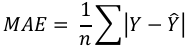
这里,Y = 实际输出值
hatY = 预测输出值。
我们可以使用 sklearn.metrics 中的 mean_absolute_error 函数来计算 MAE。
均方误差 (MSE) (Mean Square Error (MSE))
MSE 类似于 MAE,但唯一的区别是它在求和之前将实际输出值和预测输出值之差平方,而不是使用绝对值。在以下方程中可以注意到这种差异:
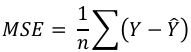
这里,Y = 实际输出值
hatY = 预测输出值。
我们可以使用 sklearn.metrics 中的 mean_squared_error 函数来计算 MSE。
R 平方 (R2) (R Squared (R2))
R 平方指标通常用于解释目的,并指示一组预测输出值与实际输出值的拟合优度。以下公式将帮助我们理解它:
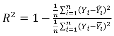
在上述方程中,分子是 MSE,分母是 Y 值中的方差。
我们可以使用 sklearn.metrics 中的 r2_score 函数来计算 R 平方值。
示例 (Example)
以下是一个简单的 Python 示例,它将向我们展示如何在回归模型上使用上面解释的性能指标:
from sklearn.metrics import r2_score
from sklearn.metrics import mean_absolute_error
from sklearn.metrics import mean_squared_error

X_actual = [5, -1, 2, 10]
Y_predic = [3.5, -0.9, 2, 9.9]

print ('R Squared =',r2_score(X_actual, Y_predic))
print ('MAE =',mean_absolute_error(X_actual, Y_predic))
print ('MSE =',mean_squared_error(X_actual, Y_predic))
输出:
R Squared = 0.9656060606060606
MAE = 0.42499999999999993
MSE = 0.5674999999999999
22. Machine Learning Algorithms – Machine
Performance
Learning with Python
Metrics
There are various metrics which we can use to evaluate the performance of ML algorithms,
classification as well as regression algorithms. We must carefully choose the metrics for
evaluating ML performance because:
How the performance of ML algorithms is measured and compared will be
dependent entirely on the metric you choose.
How you weight the importance of various characteristics in the result will be
influenced completely by the metric you choose.
Performance Metrics for Classification Problems
We have discussed classification and its algorithms in the previous chapters. Here, we are
going to discuss various performance metrics that can be used to evaluate predictions for
classification problems.
Confusion Matrix
It is the easiest way to measure the performance of a classification problem where the
output can be of two or more type of classes. A confusion matrix is nothing but a table
with two dimensions viz. “Actual” and “Predicted” and furthermore, both the dimensions
have “True Positives (TP)”, “True Negatives (TN)”, “False Positives (FP)”, “False Negatives
(FN)” as shown below:
1
Actual
0
Predicted
1
0
True Positives (TP)
False Negatives (FN)
False Positives (FP)
True Negatives (TN)
Explanation of the terms associated with confusion matrix are as follows:
True Positives (TP): It is the case when both actual class & predicted class of
data point is 1.
True Negatives (TN): It is the case when both actual class & predicted class of
data point is 0.
False Positives (FP): It is the case when actual class of data point is 0 & predicted
class of data point is 1.
137
Machine Learning with Python
False Negatives (FN): It is the case when actual class of data point is 1 &
predicted class of data point is 0.
We can use confusion_matrix function of sklearn.metrics to compute Confusion Matrix
of our classification model.
Classification Accuracy
It is most common performance metric for classification algorithms. It may be defined as
the number of correct predictions made as a ratio of all predictions made. We can easily
calculate it by confusion matrix with the help of following formula:
TP + TN
Accuracy =
TP + FP + FN + TN
We can use accuracy_score function of sklearn.metrics to compute accuracy of our
classification model.
Classification Report
This report consists of the scores of Precisions, Recall, F1 and Support. They are explained
as follows:
Precision
Precision, used in document retrievals, may be defined as the number of correct
documents returned by our ML model. We can easily calculate it by confusion matrix with
the help of following formula:
TP
Precision =
TP + FP
Recall or Sensitivity
Recall may be defined as the number of positives returned by our ML model. We can easily
calculate it by confusion matrix with the help of following formula:
TP
Recall =
TP + FN
Specificity
Specificity, in contrast to recall, may be defined as the number of negatives returned by
our ML model. We can easily calculate it by confusion matrix with the help of following
formula:
TN
Specificity =
TN + FP
138
Machine Learning with Python
Support
Support may be defined as the number of samples of the true response that lies in each
class of target values.
F1 Score
This score will give us the harmonic mean of precision and recall. Mathematically, F1 score
is the weighted average of the precision and recall. The best value of F1 would be 1 and
worst would be 0. We can calculate F1 score with the help of following formula:
F1 = 2 ∗ (precision ∗ recall) / (precision + recall)
F1 score is having equal relative contribution of precision and recall.
We can use classification_report function of sklearn.metrics to get the classification
report of our classification model.
AUC (Area Under ROC curve)
AUC (Area Under Curve)-ROC (Receiver Operating Characteristic) is a performance metric,
based on varying threshold values, for classification problems. As name suggests, ROC is
a probability curve and AUC measure the separability. In simple words, AUC-ROC metric
will tell us about the capability of model in distinguishing the classes. Higher the AUC,
better the model.
Mathematically, it can be created by plotting TPR (True Positive Rate) i.e. Sensitivity or
recall vs FPR (False Positive Rate) i.e. 1-Specificity, at various threshold values. Following
is the graph showing ROC, AUC having TPR at y-axis and FPR at x-axis:
TPR
ROC
AOC
FPR
We can use roc_auc_score function of sklearn.metrics to compute AUC-ROC.
LOGLOSS (Logarithmic Loss)
It is also called Logistic regression loss or cross-entropy loss. It basically defined on
probability estimates and measures the performance of a classification model where the
input is a probability value between 0 and 1. It can be understood more clearly by
differentiating it with accuracy. As we know that accuracy is the count of predictions
(predicted value = actual value) in our model whereas Log Loss is the amount of
uncertainty of our prediction based on how much it varies from the actual label. With the
139
Machine Learning with Python
help of Log Loss value, we can have more accurate view of the performance of our model.
We can use log_loss function of sklearn.metrics to compute Log Loss.
Example
The following is a simple recipe in Python which will give us an insight about how we can
use the above explained performance metrics on binary classification model:
from sklearn.metrics import confusion_matrix
from sklearn.metrics import accuracy_score
from sklearn.metrics import classification_report
from sklearn.metrics import roc_auc_score
from sklearn.metrics import log_loss
X_actual = [1, 1, 0, 1, 0, 0, 1, 0, 0, 0]
Y_predic = [1, 0, 1, 1, 1, 0, 1, 1, 0, 0]
results = confusion_matrix(X_actual, Y_predic)
print ('Confusion Matrix :')
print(results)
print ('Accuracy Score is',accuracy_score(X_actual, Y_predic))
print ('Classification Report : ')
print (classification_report(X_actual, Y_predic))
print('AUC-ROC:',roc_auc_score(X_actual, Y_predic))
print('LOGLOSS Value is',log_loss(X_actual, Y_predic))
Output
Confusion Matrix :
[[3 3]
[1 3]]
Accuracy Score is 0.6
Classification Report :
precision
recall
f1-score
support
0
0.75
0.50
0.60
6
1
0.50
0.75
0.60
4
micro avg
0.60
0.60
0.60
10
macro avg
0.62
0.62
0.60
10
weighted avg
0.65
0.60
0.60
10
AUC-ROC: 0.625
LOGLOSS Value is 13.815750437193334
140
Machine Learning with Python
Performance Metrics for Regression Problems
We have discussed regression and its algorithms in previous chapters. Here, we are going
to discuss various performance metrics that can be used to evaluate predictions for
regression problems.
Mean Absolute Error (MAE)
It is the simplest error metric used in regression problems. It is basically the sum of
average of the absolute difference between the predicted and actual values. In simple
words, with MAE, we can get an idea of how wrong the predictions were. MAE does not
indicate the direction of the model i.e. no indication about underperformance or
overperformance of the model. The following is the formula to calculate MAE:
1
MAE =
∑|Y − Ŷ|
n
Here, Y=Actual Output Values
And Ŷ = Predicted Output Values.
We can use mean_absolute_error function of sklearn.metrics to compute MAE.
Mean Square Error (MSE)
MSE is like the MAE, but the only difference is that the it squares the difference of actual
and predicted output values before summing them all instead of using the absolute value.
The difference can be noticed in the following equation:
1
MSE =
∑(Y − Ŷ)
n
Here, Y=Actual Output Values
And Ŷ = Predicted Output Values.
We can use mean_squared_error function of sklearn.metrics to compute MSE.
R Squared (R2)
R Squared metric is generally used for explanatory purpose and provides an indication of
the goodness or fit of a set of predicted output values to the actual output values. The
following formula will help us understanding it:
2
n 1 ∑n
i=1(Yi
−Y
̂ i )2
R =1−
1 n
n ∑i=1(Yi
−Y
̅ i )2
In the above equation, numerator is MSE and the denominator is the variance in Y values.
We can use r2_score function of sklearn.metrics to compute R squared value.
141
Machine Learning with Python
Example
The following is a simple recipe in Python which will give us an insight about how we can
use the above explained performance metrics on regression model:
from sklearn.metrics import r2_score
from sklearn.metrics import mean_absolute_error
from sklearn.metrics import mean_squared_error
X_actual = [5, -1, 2, 10]
Y_predic = [3.5, -0.9, 2, 9.9]
print ('R Squared =',r2_score(X_actual, Y_predic))
print ('MAE =',mean_absolute_error(X_actual, Y_predic))
print ('MSE =',mean_squared_error(X_actual, Y_predic))
Output
R Squared = 0.9656060606060606
MAE = 0.42499999999999993
MSE = 0.5674999999999999