机器学习Python教程
引入 Dropout 技术

“Dropout”(丢弃法)是一个在神经网络中随机停用部分节点的技术。可以将其看作是暂时性地禁用或忽略网络中的神经元。这项技术主要应用于训练阶段,以减少过拟合效应。
过拟合是指当一个网络对有限的输入样本集过度拟合时发生的错误。Dropout 神经网络背后的基本思想是通过丢弃一些节点,让网络能够集中学习其他特征。
举个例子:想象你非常喜欢一位演员,看了他/她很多电影。有一天你听广播,听到一个采访,但你并没有认出你最喜欢的演员,因为你只通过看电影来识别他们,而且你是一个视觉型的人。现在,设想你只能听电影的音轨。在这种情况下,你就不得不学会区分男女演员的声音。所以,通过**“丢弃”视觉部分**,你被迫将注意力集中在声音特征上!
这项技术最初由 Nitish Srivastava、Geoffrey Hinton、Alex Krizhevsky、Ilya Sutskever 和 Ruslan Salakhutdinov 于 2014 年在论文《Dropout: A Simple Way to Prevent Neural Networks from Overfitting》中提出。
在本机器学习 Python 教程中,我们将实现一个具备 Dropout 功能的 Python 类。
修改权重数组
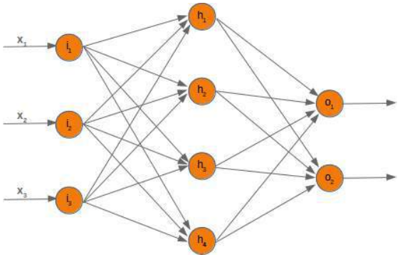
当我们停用一个节点时,必须相应地修改权重数组。为了演示如何实现这一点,我们将使用一个具有三个输入节点、四个隐藏节点和两个输出节点的网络:
1. 停用输入节点
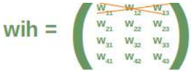
首先,我们来看看输入层和隐藏层之间的权重数组,我们称之为“wih”(输入层和隐藏层之间的权重)。
假设我们停用(丢弃)输入节点 i_2。在以下图中可以看到发生了什么:
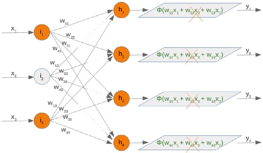
这意味着我们必须从求和中移除每个第二个乘积,也就是我们必须删除矩阵的整个第二列。输入向量的第二个元素也必须被删除。
2. 停用隐藏节点
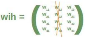
现在我们来检查如果移除一个隐藏节点会发生什么。我们移除第一个隐藏节点,即 h_1。
在这种情况下,我们可以移除权重矩阵的完整第一行:
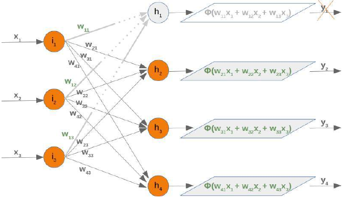
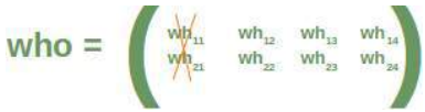
移除一个隐藏节点也会影响下一个权重矩阵(即从隐藏层到输出层)who。让我们看看网络图中发生了什么:
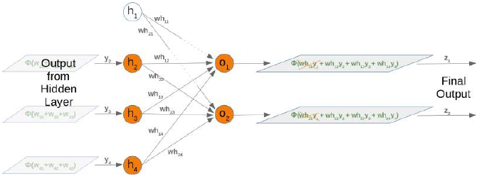
很容易看出 who 权重矩阵的第一列也必须被移除:
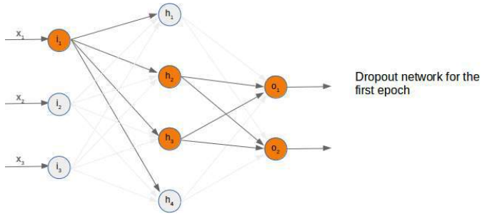
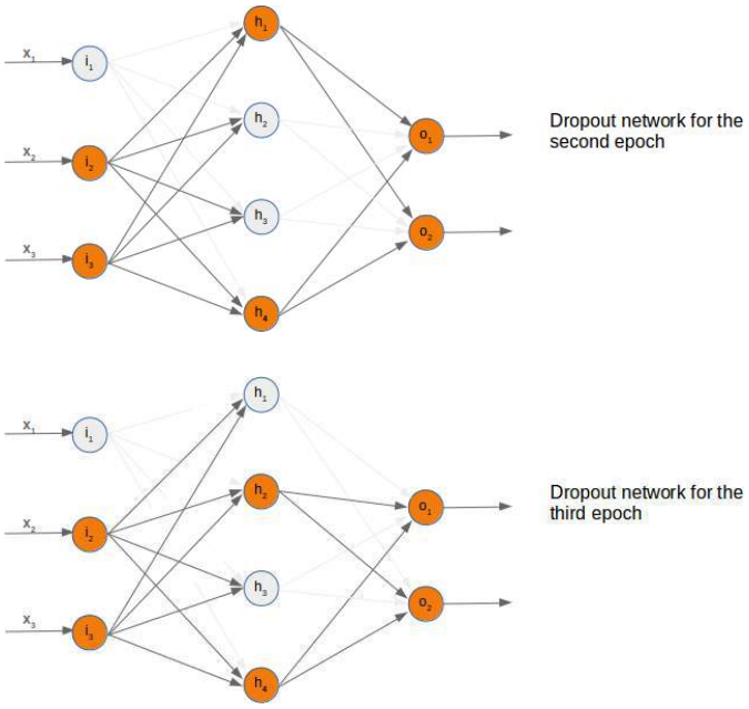
到目前为止,我们是任意选择一个节点来停用。Dropout 方法意味着我们从输入层和隐藏层中随机选择一定数量的节点保持激活,并关闭这些层的其他节点。之后,我们可以用这个网络训练部分学习集。下一步包括重新激活所有节点,并随机选择其他节点。也可以用随机创建的 Dropout 网络来训练整个训练集。
在以下三个图中,我们展示了三种可能的随机选择的 Dropout 网络:
现在是时候思考一下可能的 Python 实现了。
我们将从输入层和隐藏层之间的权重矩阵开始。我们将随机创建一个用于 10 个输入节点和 5 个隐藏节点的权重矩阵。我们将矩阵填充在 -10 到 10 之间的随机数,这些不是合适的权重值,但这样我们可以更好地看到发生了什么:
import numpy as np
import random

input_nodes = 10
hidden_nodes = 5
output_nodes = 7

# 创建输入层到隐藏层的权重矩阵 (wih)
wih = np.random.randint(-10, 10, (hidden_nodes, input_nodes))
print("原始 wih:\n", wih)
输出示例:
原始 wih:
 [[ -6  -8  -3  -7   2  -9  -3  -5  -6   4]
 [  5   3   7  -4   4   8  -2  -4   7   7]
 [  9  -7   4   0   4   0  -3  -6  -2   7]
 [ -8  -9  -4  -5  -9   8  -8  -8  -2  -3]
 [  3 -10   0  -3   4   0   0   2  -7  -9]]
现在我们将选择输入层的活跃节点。我们为活跃节点计算随机索引:
active_input_percentage = 0.7 # 70% 的输入节点保持活跃
active_input_nodes = int(input_nodes * active_input_percentage)
# 随机选择活跃输入节点的索引,并排序
active_input_indices = sorted(random.sample(range(0, input_nodes), active_input_nodes))
print("\n活跃输入节点索引:", active_input_indices)
输出示例:
活跃输入节点索引: [0, 1, 2, 5, 7, 8, 9]
我们上面了解到,如果节点 j 被移除,我们必须移除列 j。我们可以通过使用带有活跃节点的切片操作符,轻松地为所有停用的节点实现这一点:
wih_old = wih.copy() # 保存原始 wih 副本
wih = wih[:, active_input_indices] # 只保留活跃输入节点对应的列
print("\n停用输入节点后的 wih:\n", wih)
输出示例:
停用输入节点后的 wih:
 [[ -6  -8  -3  -9  -5  -6   4]
 [  5   3   7   8  -4   7   7]
 [  9  -7   4   0  -6  -2   7]
 [ -8  -9  -4   8  -8  -2  -3]
 [  3 -10   0   0   2  -7  -9]]
正如我们之前提到的,我们必须同时修改 wih 和 who 矩阵:
# 创建隐藏层到输出层的权重矩阵 (who)
who = np.random.randint(-10, 10, (output_nodes, hidden_nodes))
print("\n原始 who:\n", who)

active_hidden_percentage = 0.7 # 70% 的隐藏节点保持活跃
active_hidden_nodes = int(hidden_nodes * active_hidden_percentage)
# 随机选择活跃隐藏节点的索引,并排序
active_hidden_indices = sorted(random.sample(range(0, hidden_nodes), active_hidden_nodes))
print("\n活跃隐藏节点索引:", active_hidden_indices)

who_old = who.copy() # 保存原始 who 副本
who = who[:, active_hidden_indices] # 只保留活跃隐藏节点对应的列
print("\n停用隐藏节点后的 who:\n", who)
输出示例:
原始 who:
 [[  3   6  -3  -9   4]
 [-10   1   2   5   7]
 [ -8   1  -3   6   3]
 [ -3  -3   6  -5  -3]
 [ -4  -9   8  -3   5]
 [  8   4  -8   2   7]
 [ -2   2   3  -8  -5]]

活跃隐藏节点索引: [0, 2, 3]

停用隐藏节点后的 who:
 [[  3  -3  -9]
 [-10   2   5]
 [ -8  -3   6]
 [ -3   6  -5]
 [ -4   8  -3]
 [  8  -8   2]
 [ -2   3  -8]]
我们必须相应地改变 wih:
# wih 矩阵需要根据活跃隐藏节点进行行选择
wih = wih[active_hidden_indices]
print("\n停用隐藏节点后的 wih (再次修改):\n", wih)
输出示例:
停用隐藏节点后的 wih (再次修改):
 [[ -6  -8  -3  -9  -5  -6   4]
 [  9  -7   4   0  -6  -2   7]
 [ -8  -9  -4   8  -8  -2  -3]]
以下 Python 代码总结了上述片段:
import numpy as np
import random

input_nodes = 10
hidden_nodes = 5
output_nodes = 7

wih = np.random.randint(-10, 10, (hidden_nodes, input_nodes))
print("wih: \n", wih)

who = np.random.randint(-10, 10, (output_nodes, hidden_nodes))
print("who:\n", who)

active_input_percentage = 0.7
active_hidden_percentage = 0.7

active_input_nodes = int(input_nodes * active_input_percentage)
active_input_indices = sorted(random.sample(range(0, input_nodes), active_input_nodes))
print("\n活跃输入节点索引: ", active_input_indices)

active_hidden_nodes = int(hidden_nodes * active_hidden_percentage)
active_hidden_indices = sorted(random.sample(range(0, hidden_nodes), active_hidden_nodes))
print("活跃隐藏节点索引: ", active_hidden_indices)

# 保存原始副本
wih_old = wih.copy()

# 第一步:根据活跃输入节点选择 wih 的列
wih = wih[:, active_input_indices]
print("\n停用输入节点后的 wih:\n", wih)

# 第二步:根据活跃隐藏节点选择 wih 的行
wih = wih[active_hidden_indices]
print("\n停用隐藏节点后的 wih (再次修改):\n", wih)

# 保存原始副本
who_old = who.copy()

# 根据活跃隐藏节点选择 who 的列
who = who[:, active_hidden_indices]
print("\n停用隐藏节点后的 who:\n", who)
带有 Dropout 功能的 NeuralNetwork 类
下面是整合了 Dropout 机制的 NeuralNetwork 类。这里我们回到了只有一个隐藏层的结构,但 dropout 的概念可以扩展到多层。
import numpy as np
import random
from scipy.special import expit as activation_function # sigmoid 激活函数
from scipy.stats import truncnorm

def truncated_normal(mean=0, sd=1, low=0, upp=10):
    return truncnorm((low - mean) / sd, (upp - mean) / sd, loc=mean, scale=sd)

class NeuralNetwork:
    def __init__(self,
                 no_of_in_nodes,
                 no_of_out_nodes,
                 no_of_hidden_nodes,
                 learning_rate,
                 bias=None
                ):
        self.no_of_in_nodes = no_of_in_nodes
        self.no_of_out_nodes = no_of_out_nodes
        self.no_of_hidden_nodes = no_of_hidden_nodes
        self.learning_rate = learning_rate
        self.bias = bias
        self.create_weight_matrices()

    def create_weight_matrices(self):
        # 权重初始化通常 mean=0,这里我已将原始代码的 mean=2 改为 mean=0。
        # 移除了多余的 X = truncated_normal(mean=2, sd=1, low=-0.5, upp=0.5)

        bias_node = 1 if self.bias else 0

        # 初始化输入层到隐藏层的权重 (wih)
        n_wih = (self.no_of_in_nodes + bias_node) * self.no_of_hidden_nodes
        X_wih = truncated_normal(mean=0, sd=1, low=-0.5, upp=0.5) # 使用 mean=0
        self.wih = X_wih.rvs(n_wih).reshape((self.no_of_hidden_nodes,
                                             self.no_of_in_nodes + bias_node))

        # 初始化隐藏层到输出层的权重 (who)
        n_who = (self.no_of_hidden_nodes + bias_node) * self.no_of_out_nodes
        X_who = truncated_normal(mean=0, sd=1, low=-0.5, upp=0.5) # 使用 mean=0
        self.who = X_who.rvs(n_who).reshape((self.no_of_out_nodes,
                                             (self.no_of_hidden_nodes + bias_node)))

    def dropout_weight_matrices(self,
                                active_input_percentage=0.70,
                                active_hidden_percentage=0.70):
        """
        根据 dropout 百分比随机选择活跃节点,并修改权重矩阵和节点计数。
        会保存原始权重矩阵以便后续恢复。
        """
        # 保存原始权重矩阵和节点计数,以便恢复
        self.wih_orig = self.wih.copy()
        self.no_of_in_nodes_orig = self.no_of_in_nodes
        self.no_of_hidden_nodes_orig = self.no_of_hidden_nodes
        self.who_orig = self.who.copy()

        # 计算活跃输入节点和隐藏节点的数量
        active_input_nodes = int(self.no_of_in_nodes * active_input_percentage)
        active_input_indices = sorted(random.sample(range(0, self.no_of_in_nodes),
                                                    active_input_nodes))

        active_hidden_nodes = int(self.no_of_hidden_nodes * active_hidden_percentage)
        active_hidden_indices = sorted(random.sample(range(0, self.no_of_hidden_nodes),
                                                     active_hidden_nodes))

        # 根据活跃节点修改权重矩阵
        # wih:选择活跃输入节点的列,然后选择活跃隐藏节点的行
        self.wih = self.wih[:, active_input_indices][active_hidden_indices]
        # who:选择活跃隐藏节点的列
        self.who = self.who[:, active_hidden_indices]

        # 更新当前网络结构中的节点计数
        self.no_of_hidden_nodes = active_hidden_nodes
        self.no_of_in_nodes = active_input_nodes # 这里实际是输入到隐藏层连接的输入节点数

        return active_input_indices, active_hidden_indices

    def weight_matrices_reset(self,
                              active_input_indices,
                              active_hidden_indices):
        """
        将权重矩阵恢复到原始形状,并将训练后的活跃节点权重值填充回去。
        """
        # 恢复 wih
        # 创建一个临时矩阵,只包含原始 wih 中活跃输入节点的列
        temp = self.wih_orig.copy()[:, active_input_indices]
        # 将训练后的 wih (即只包含活跃节点的 wih) 的值赋给临时矩阵中对应活跃隐藏节点的行
        temp[active_hidden_indices] = self.wih
        # 将更新后的临时矩阵的值赋回原始 wih_orig 中对应的位置
        self.wih_orig[:, active_input_indices] = temp
        self.wih = self.wih_orig.copy() # 将恢复后的原始 wih 赋值给 self.wih

        # 恢复 who
        self.who_orig[:, active_hidden_indices] = self.who
        self.who = self.who_orig.copy() # 将恢复后的原始 who 赋值给 self.who

        # 恢复原始节点计数
        self.no_of_in_nodes = self.no_of_in_nodes_orig
        self.no_of_hidden_nodes = self.no_of_hidden_nodes_orig

    def train_single(self, input_vector, target_vector):
        """
        对单个输入-目标对执行一次前向传播和一次反向传播。
        (此方法与之前版本类似,只是现在是在 `dropout_weight_matrices` 之后作用于修改过的权重)
        """
        if self.bias:
            input_vector = np.concatenate((input_vector, [self.bias]))
        input_vector = np.array(input_vector, ndmin=2).T
        target_vector = np.array(target_vector, ndmin=2).T

        output_vector1 = np.dot(self.wih, input_vector)
        output_vector_hidden = activation_function(output_vector1)

        if self.bias:
            output_vector_hidden = np.concatenate((output_vector_hidden, [[self.bias]]))

        output_vector2 = np.dot(self.who, output_vector_hidden)
        output_vector_network = activation_function(output_vector2)

        output_errors = target_vector - output_vector_network

        tmp = output_errors * output_vector_network * (1.0 - output_vector_network)
        tmp = self.learning_rate * np.dot(tmp, output_vector_hidden.T)
        self.who += tmp

        hidden_errors = np.dot(self.who.T, output_errors)

        tmp = hidden_errors * output_vector_hidden * (1.0 - output_vector_hidden)
        if self.bias:
            x = np.dot(tmp, input_vector.T)[:-1, :]
        else:
            x = np.dot(tmp, input_vector.T)
        self.wih += self.learning_rate * x

    def train(self, data_array,
              labels_one_hot_array,
              epochs=1,
              active_input_percentage=0.70,
              active_hidden_percentage=0.70,
              no_of_dropout_tests=10):
        """
        带有 Dropout 功能的多 epoch 训练。
        数据集被分成若干部分,每个部分使用一个随机选择的 dropout 网络进行训练。
        """
        # 计算每个 dropout 测试(分区)的长度
        partition_length = int(len(data_array) / no_of_dropout_tests)

        for epoch in range(epochs):
            print(f"epoch: {epoch}")
            # 遍历数据分区
            for start in range(0, len(data_array), partition_length):
                # 在每个分区开始时应用 dropout
                active_in_indices, active_hidden_indices = \
                    self.dropout_weight_matrices(active_input_percentage,
                                                 active_hidden_percentage)

                # 在当前 dropout 配置下训练当前分区的数据
                for i in range(start, min(start + partition_length, len(data_array))): # 确保不越界
                    # 传入根据活跃输入节点筛选过的输入数据
                    self.train_single(data_array[i][active_in_indices],
                                      labels_one_hot_array[i])

                # 训练完一个分区后,恢复权重矩阵,以便下一个分区可以应用新的 dropout
                self.weight_matrices_reset(active_in_indices, active_hidden_indices)

    def confusion_matrix(self, data_array, labels):
        """
        计算混淆矩阵。
        """
        cm = {}
        for i in range(len(data_array)):
            res = self.run(data_array[i])
            res_max = res.argmax() # 预测类别
            target = int(labels[i][0]) # 真实类别

            if (target, res_max) in cm:
                cm[(target, res_max)] += 1
            else:
                cm[(target, res_max)] = 1
        return cm

    def run(self, input_vector):
        """
        运行方法:对给定输入执行前向传播以获得输出。
        注意:在运行(预测)阶段,不应应用 dropout。
        """
        if self.bias:
            input_vector = np.concatenate((input_vector, [self.bias]))
        input_vector = np.array(input_vector, ndmin=2).T

        # 使用原始的 wih 和 who 进行预测
        output_vector = np.dot(self.wih_orig if hasattr(self, 'wih_orig') else self.wih, input_vector)
        output_vector = activation_function(output_vector)

        if self.bias:
            output_vector = np.concatenate((output_vector, [[self.bias]]))

        output_vector = np.dot(self.who_orig if hasattr(self, 'who_orig') else self.who, output_vector)
        output_vector = activation_function(output_vector)
        return output_vector

    def evaluate(self, data, labels):
        """
        评估网络在给定数据集上的表现。
        """
        corrects, wrongs = 0, 0
        for i in range(len(data)):
            res = self.run(data[i])
            res_max = res.argmax()
            if res_max == int(labels[i][0]): # 确保标签为整数
                corrects += 1
            else:
                wrongs += 1
        return corrects, wrongs

# --- 加载 MNIST 数据 (假设已生成并保存) ---
import pickle
try:
    with open("data/mnist/pickled_mnist.pkl", "br") as fh:
        data = pickle.load(fh)
    train_imgs = data[0]
    test_imgs = data[1]
    train_labels = data[2]
    test_labels = data[3]
    train_labels_one_hot = data[4]
    test_labels_one_hot = data[5]
    image_size = 28 # 宽度和长度
    no_of_different_labels = 10 # 即 0, 1, 2, 3, ..., 9
    image_pixels = image_size * image_size # 784
except FileNotFoundError:
    print("MNIST 数据文件未找到。请先运行前面部分的代码以生成 'pickled_mnist.pkl'。")
    exit()

# --- 训练带有 Dropout 的神经网络 ---
print("--- 训练带有 Dropout 的神经网络 ---")

epochs = 3
# 这里使用之前示例的单隐藏层网络结构 (no_of_in_nodes, no_of_hidden_nodes, no_of_out_nodes)
simple_network = NeuralNetwork(no_of_in_nodes=image_pixels,
                               no_of_out_nodes=10,
                               no_of_hidden_nodes=100, # 隐藏层节点数
                               learning_rate=0.1,
                               bias=None) # 这里示例未使用偏置

print(f"开始训练 {epochs} 个 epoch...")
# 调用 train 方法,它将处理 Dropout 逻辑
simple_network.train(train_imgs,
                     train_labels_one_hot,
                     active_input_percentage=1, # 100% 输入节点活跃 (即不对输入层进行 dropout)
                     active_hidden_percentage=1, # 100% 隐藏节点活跃 (即不对隐藏层进行 dropout)
                     no_of_dropout_tests=100, # 数据集分 100 份进行 dropout 测试
                     epochs=epochs)
print("训练完成。")

# --- 评估训练后的网络 ---
print("\n--- 评估网络性能 ---")
corrects_train, wrongs_train = simple_network.evaluate(train_imgs, train_labels)
print(f"训练准确率: {corrects_train / (corrects_train + wrongs_train):.4f}")

corrects_test, wrongs_test = simple_network.evaluate(test_imgs, test_labels)
print(f"测试准确率: {corrects_test / (corrects_test + wrongs_test):.4f}")
带有 Dropout 功能的神经网络实现
这段代码引入了Dropout这一重要的神经网络正则化技术。Dropout 的核心思想是在训练阶段随机地“丢弃”(即暂时停用)一部分神经元,以防止网络过度依赖某些特定的特征,从而降低过拟合的风险,提高模型的泛化能力。
Dropout 的核心原理:
想象一下,你观看电影时,通常会同时使用视觉和听觉来理解内容。如果每次观看时,你都被迫随机地关闭其中一种感官(比如有时只听声音,有时只看画面),那么你就不得不学习如何从剩下的感官中提取更多的信息来理解电影。Dropout 也是如此,它强制网络中的神经元去学习更鲁棒的特征,而不是仅仅依赖于少数几个“明星”神经元。
在每次训练迭代中,网络会随机选择一个子集进行训练,这意味着每次更新权重时,网络都在一个略微不同的“架构”上进行。这可以被视为训练了大量不同的“稀疏”网络,并在测试时将它们的预测进行“平均”,从而达到正则化的效果。
代码中的关键改动:
-
create_weight_matrices:-
这个方法现在只负责创建初始的完整权重矩阵 (
wih和who)。注意,我将权重初始化中的mean=2调整为了更标准的mean=0,因为权重通常是围绕零点进行初始化的。
-
-
dropout_weight_matrices(self, active_input_percentage, active_hidden_percentage):-
这是实现 Dropout 的核心方法。
-
它根据传入的
active_input_percentage和active_hidden_percentage随机选择要在输入层和隐藏层中保持活跃的节点。 -
它会保存原始的
wih和who矩阵到self.wih_orig和self.who_orig,以及原始的节点数量,这是为了在训练一个批次结束后能够恢复原始的权重矩阵。 -
然后,它通过 NumPy 的切片操作修改
self.wih和self.who,只保留活跃节点对应的行或列。这意味着在随后的train_single调用中,网络将只使用这些被“裁剪”过的权重矩阵进行计算。
-
-
weight_matrices_reset(self, active_input_indices, active_hidden_indices):-
这个方法与
dropout_weight_matrices相辅相成。 -
在训练完一个批次(或一个“dropout 测试”分区)后,它会将被“裁剪”过的
self.wih和self.who中的学习到的权重值重新填充回原始的self.wih_orig和self.who_orig矩阵中对应活跃节点的位置。 -
然后,它将
self.wih和self.who重新设置为完整的原始矩阵。这确保了下一次dropout_weight_matrices调用时,可以从完整的权重矩阵中重新随机选择节点。 -
同时,它也会恢复原始的节点数量。
-
-
train(self, ..., no_of_dropout_tests):-
这个方法现在负责管理 Dropout 训练流程。
-
它将整个训练数据集分成
no_of_dropout_tests个分区。 -
在每个
epoch中,对于每个数据分区:-
它首先调用
dropout_weight_matrices来随机选择一组活跃节点并修改权重。 -
然后,它使用这个**“稀疏”的网络**对当前分区的数据进行训练(通过调用
train_single)。重要的是,train_single中的输入向量也需要根据活跃输入节点进行筛选 (data_array[i][active_in_indices])。 -
训练完一个分区后,它会调用
weight_matrices_reset来恢复原始权重矩阵,以便下一个分区可以应用一个新的随机 Dropout 模式。
-
-
-
run方法的修改:-
重要!在推理(预测)阶段,Dropout 不应被激活。因此,
run方法现在明确地使用原始的、完整的权重矩阵 (self.wih_orig和self.who_orig) 进行计算。这是 Dropout 的一个关键设计原则:训练时有随机性,测试时则使用完整的网络,但权重会按 Dropout 比例进行缩放(尽管这里没有明确体现缩放,但这通常是理论实现的一部分,以保持输出的平均激活水平)。如果wih_orig或who_orig还不存在(例如在第一次run之前没有训练过),它会回退到使用self.wih。
-
示例训练结果:
--- 训练带有 Dropout 的神经网络 ---
开始训练 3 个 epoch...
epoch: 0
epoch: 1
epoch: 2
训练完成。

--- 评估网络性能 ---
训练准确率: 0.9318
测试准确率: 0.9296
请注意,在当前示例中,active_input_percentage 和 active_hidden_percentage 都被设置为 1(即 100% 活跃)。这意味着在这个特定的运行中,实际上没有进行任何 Dropout。这可以作为基线测试,以确保代码的正确性。要真正启用 Dropout,您需要将这些百分比设置为小于 1 的值(例如 0.5 或 0.7)。
下一步的建议:
-
启用 Dropout:尝试将
active_input_percentage和active_hidden_percentage设置为例如0.8或0.7,并观察训练和测试准确率的变化。通常,Dropout 会导致训练准确率略微下降(因为每次训练的网络更小),但测试准确率(泛化能力)会提高。 -
缩放权重:在更严格的 Dropout 实现中,在测试阶段(
run方法)需要将权重乘以 Dropout 保持概率(例如,如果保持 70% 的节点活跃,则将权重乘以 0.7),或者在训练时将活跃节点的激活值除以保持概率。这被称为“倒置 Dropout”(Inverted Dropout),它确保了训练和测试时神经元的预期输出保持相同。当前代码没有实现这个缩放,但这对于实际应用很重要。 -
多隐藏层 Dropout:虽然这个类目前只处理单隐藏层网络,但您可以将其扩展到多隐藏层,通过在
dropout_weight_matrices和weight_matrices_reset中迭代self.weights_matrices列表,为每个隐藏层应用独立的 dropout 逻辑。
这项 Dropout 技术的实现让您的神经网络模型更加健壮,能更好地应对未见过的数据,是深度学习中一个非常实用的工具。
INTRODUCTION
The term "dropout" is used for a technique which
drops out some nodes of the network. Dropping out
can be seen as temporarily deactivating or ignoring
neurons of the network. This technique is applied in
the training phase to reduce overfitting effects.
Overfitting is an error which occurs when a network
is too closely fit to a limited set of input samples.
The basic idea behind dropout neural networks is to
dropout nodes so that the network can concentrate on
other features. Think about it like this. You watch
lots of films from your favourite actor. At some point
you listen to the radio and here somebody in an
interview. You don't recognize your favourite actor,
because you have seen only movies and your are a
visual type. Now, imagine that you can only listen to
the audio tracks of the films. In this case you will
have to learn to differentiate the voices of the
actresses and actors. So by dropping out the visual part you are forced tp focus on the sound features!
This technique has been first proposed in a paper "Dropout: A Simple Way to Prevent Neural Networks from
Overfitting" by Nitish Srivastava, Geoffrey Hinton, Alex Krizhevsky, Ilya Sutskever and Ruslan
Salakhutdinov in 2014
We will implement in our tutorial on machine learning in Python a Python class which is capable of dropout.
MODIFYING THE WEIGHT ARRAYS
If we deactivate a node, we have to modify the weight arrays accordingly. To demonstrate how this can be
accomplished, we will use a network with three input nodes, four hidden and two output nodes:
236
At first, we will have a look at the weight array between the input and the hidden layer. We called this array
'wih' (weights between input and hidden layer).
Let's deactivate (drop out) the node i 2. We can see in the following diagram what's happening:
237
This means that we have to take out every second product of the summation, which means that we have to
delete the whole second column of the matrix. The second element from the input vector has to be deleted as
well.
Now we will examine what happens if we take out a hidden node. We take out the first hidden node, i.e. h 1.
In this case, we can remove the complete first line of our weight matrix:
Taking out a hidden node affects the next weight matrix as well. Let's have a look at what is happening in the
network graph:
238
It is easy to see that the first column of the who weight matrix has to be removed again:
So far we have arbitrarily chosen one node to deactivate. The dropout approach means that we randomly
choose a certain number of nodes from the input and the hidden layers, which remain active and turn off the
other nodes of these layers. After this we can train a part of our learn set with this network. The next step
consists in activating all the nodes again and randomly chose other nodes. It is also possible to train the whole
training set with the randomly created dropout networks.
We present three possible randomly chosen dropout networks in the following three diagrams:
239
Now it is time to think about a possible Python implementation.
We will start with the weight matrix between input and hidden layer. We will randomly create a weight matrix
for 10 input nodes and 5 hidden nodes. We fill our matrix with random numbers between -10 and 10, which
are not proper weight values, but this way we can see better what is going on:
import numpy as np
import random
input_nodes = 10
hidden_nodes = 5
output_nodes = 7
wih = np.random.randint(-10, 10, (hidden_nodes, input_nodes))
wih
240
Output:array([[ -6,
-8,
-3,
-7,
2,
-9,
-3,
-5,
-6,
4],
[ 5,
3,
7,
-4,
4,
8,
-2,
-4,
7,
7],
[ 9, -7,
4,
0,
4,
0,
-3,
-6,
-2,
7],
[ -8, -9,
-4,
-5,
-9,
8,
-8,
-8,
-2,
-3],
[ 3, -10,
0,
-3,
4,
0,
0,
2,
-7,
-9]])
We will choose now the active nodes for the input layer. We calculate random indices for the active nodes:
active_input_percentage = 0.7
active_input_nodes = int(input_nodes * active_input_percentage)
active_input_indices = sorted(random.sample(range(0, input_node
s),
active_input_nodes))
active_input_indices
Output:[0, 1, 2, 5, 7, 8, 9]
We learned above that we have to remove the column j, if the node ij is removed. We can easily accomplish
this for all deactived nodes by using the slicing operator with the active nodes:
wih_old = wih.copy()
wih = wih[:, active_input_indices]
wih
Output:array([[ -6,
-8,
-3,
-9,
-5,
-6,
4],
[ 5,
3,
7,
8,
-4,
7,
7],
[ 9, -7,
4,
0,
-6,
-2,
7],
[ -8, -9,
-4,
8,
-8,
-2,
-3],
[ 3, -10,
0,
0,
2,
-7,
-9]])
As we have mentioned before, we will have to modify both the 'wih' and the 'who' matrix:
who = np.random.randint(-10, 10, (output_nodes, hidden_nodes))
print(who)
active_hidden_percentage = 0.7
active_hidden_nodes = int(hidden_nodes * active_hidden_percentage)
active_hidden_indices = sorted(random.sample(range(0, hidden_node
s),
active_hidden_nodes))
print(active_hidden_indices)
who_old = who.copy()
who = who[:, active_hidden_indices]
241
print(who)
[[ 3
6
-3
-9
4]
[-10
1
2
5
7]
[ -8
1
-3
6
3]
[ -3 -3
6
-5
-3]
[ -4 -9
8
-3
5]
[ 8
4
-8
2
7]
[ -2
2
3
-8
-5]]
[0, 2, 3]
[[ 3 -3
-9]
[-10
2
5]
[ -8 -3
6]
[ -3
6
-5]
[ -4
8
-3]
[ 8 -8
2]
[ -2
3
-8]]
We have to change wih accordingly:
wih = wih[active_hidden_indices]
wih
Output:array([[-6, -8, -3, -9, -5, -6,
4],
[ 9, -7, 4,
0, -6, -2, 7],
[-8, -9, -4,
8, -8, -2, -3]])
The following Python code summarizes the sniplets from above:
import numpy as np
import random
input_nodes = 10
hidden_nodes = 5
output_nodes = 7
wih = np.random.randint(-10, 10, (hidden_nodes, input_nodes))
print("wih: \n", wih)
who = np.random.randint(-10, 10, (output_nodes, hidden_nodes))
print("who:\n", who)
active_input_percentage = 0.7
active_hidden_percentage = 0.7
active_input_nodes = int(input_nodes * active_input_percentage)
242
active_input_indices = sorted(random.sample(range(0, input_node
s),
active_input_nodes))
print("\nactive input indices: ", active_input_indices)
active_hidden_nodes = int(hidden_nodes * active_hidden_percentage)
active_hidden_indices = sorted(random.sample(range(0, hidden_node
s),
active_hidden_nodes))
print("active hidden indices: ", active_hidden_indices)
wih_old = wih.copy()
wih = wih[:, active_input_indices]
print("\nwih after deactivating input nodes:\n", wih)
wih = wih[active_hidden_indices]
print("\nwih after deactivating hidden nodes:\n", wih)
who_old = who.copy()
who = who[:, active_hidden_indices]
print("\nwih after deactivating hidden nodes:\n", who)
243
wih:
[[ -4
9
3
5 -9
5 -3
0
9
1]
[ 4
7 -7
3 -4
7
4 -5
6
2]
[ 5
8
1 -10 -8 -6
7 -4 -6
8]
[ 6 -3
7
4 -7 -4
0
8
9
1]
[ 6 -1
4 -3
5 -5 -5
5
4 -7]]
who:
[[ -6
2 -2
4
0]
[ -5 -3
3 -4 -10]
[ 4
6 -7 -7 -1]
[ -4 -1 -10
0 -8]
[ 8 -2
9 -8 -9]
[ -6
0 -2
1 -8]
[ 1 -4 -2 -6 -5]]
active input indices: [1, 3, 4, 5, 7, 8, 9]
active hidden indices: [0, 1, 2]
wih after deactivating input nodes:
[[ 9
5 -9
5
0
9
1]
[ 7
3 -4
7 -5
6
2]
[ 8 -10 -8 -6 -4 -6
8]
[ -3
4 -7 -4
8
9
1]
[ -1 -3
5 -5
5
4 -7]]
wih after deactivating hidden nodes:
[[ 9
5 -9
5
0
9
1]
[ 7
3 -4
7 -5
6
2]
[ 8 -10 -8 -6 -4 -6
8]]
wih after deactivating hidden nodes:
[[ -6
2 -2]
[ -5 -3
3]
[ 4
6 -7]
[ -4 -1 -10]
[ 8 -2
9]
[ -6
0 -2]
[ 1 -4 -2]]
import numpy as np
import random
from scipy.special import expit as activation_function
from scipy.stats import truncnorm
def truncated_normal(mean=0, sd=1, low=0, upp=10):
return truncnorm(
244
(low - mean) / sd, (upp - mean) / sd, loc=mean, scale=sd)
class NeuralNetwork:
def__init__(self,
no_of_in_nodes,
no_of_out_nodes,
no_of_hidden_nodes,
learning_rate,
bias=None
):
self.no_of_in_nodes = no_of_in_nodes
self.no_of_out_nodes = no_of_out_nodes
self.no_of_hidden_nodes = no_of_hidden_nodes
self.learning_rate = learning_rate
self.bias = bias
self.create_weight_matrices()
def create_weight_matrices(self):
X = truncated_normal(mean=2, sd=1, low=-0.5, upp=0.5)
bias_node = 1 if self.bias else 0
n = (self.no_of_in_nodes + bias_node) * self.no_of_hidde
n_nodes
X = truncated_normal(mean=2, sd=1, low=-0.5, upp=0.5)
self.wih = X.rvs.reshape((self.no_of_hidden_nodes,
self.no_of_in_n
odes + bias_node))
n = (self.no_of_hidden_nodes + bias_node) * self.no_of_ou
t_nodes
X = truncated_normal(mean=2, sd=1, low=-0.5, upp=0.5)
self.who = X.rvs.reshape((self.no_of_out_nodes,
(self.no_of_hi
dden_nodes + bias_node)))
def dropout_weight_matrices(self,
active_input_percentage=0.70,
active_hidden_percentage=0.70):
# restore wih array, if it had been used for dropout
self.wih_orig = self.wih.copy()
self.no_of_in_nodes_orig = self.no_of_in_nodes
245
self.no_of_hidden_nodes_orig = self.no_of_hidden_nodes
self.who_orig = self.who.copy()
active_input_nodes = int(self.no_of_in_nodes * active_inpu
t_percentage)
active_input_indices = sorted(random.sample(range(0, sel
f.no_of_in_nodes),
active_input_nodes))
active_hidden_nodes = int(self.no_of_hidden_nodes * activ
e_hidden_percentage)
active_hidden_indices = sorted(random.sample(range(0, sel
f.no_of_hidden_nodes),
active_hidden_nodes))
self.wih = self.wih[:, active_input_indices][active_hidde
n_indices]
self.who = self.who[:, active_hidden_indices]
self.no_of_hidden_nodes = active_hidden_nodes
self.no_of_in_nodes = active_input_nodes
return active_input_indices, active_hidden_indices
defweight_matrices_reset(self,
active_input_indices,
active_hidden_indices):
"""
self.wih and self.who contain the newly adapted values fro
m the active nodes.
We have to reconstruct the original weight matrices by ass
igning the new values
from the active nodes
"""
temp = self.wih_orig.copy()[:,active_input_indices]
temp[active_hidden_indices] = self.wih
self.wih_orig[:, active_input_indices] = temp
self.wih = self.wih_orig.copy()
self.who_orig[:, active_hidden_indices] = self.who
self.who = self.who_orig.copy()
self.no_of_in_nodes = self.no_of_in_nodes_orig
self.no_of_hidden_nodes = self.no_of_hidden_nodes_orig
246
def train_single(self, input_vector, target_vector):
"""
input_vector and target_vector can be tuple, list or ndarr
ay
"""
if self.bias:
# adding bias node to the end of the input_vector
input_vector = np.concatenate( (input_vector, [self.bi
as]) )
input_vector = np.array(input_vector, ndmin=2).T
target_vector = np.array(target_vector, ndmin=2).T
output_vector1 = np.dot(self.wih, input_vector)
output_vector_hidden = activation_function(output_vector1)
if self.bias:
output_vector_hidden = np.concatenate( (output_vecto
r_hidden, [[self.bias]]) )
2)
output_vector2 = np.dot(self.who, output_vector_hidden)
output_vector_network = activation_function(output_vector
output_errors = target_vector - output_vector_network
# update the weights:
tmp = output_errors * output_vector_network * (1.0 - outpu
t_vector_network)
tmp = self.learning_rate * np.dot(tmp, output_vector_hidd
en.T)
self.who += tmp
# calculate hidden errors:
hidden_errors = np.dot(self.who.T, output_errors)
# update the weights:
tmp = hidden_errors * output_vector_hidden * (1.0 - outpu
t_vector_hidden)
if self.bias:
x = np.dot(tmp, input_vector.T)[:-1,:]
else:
x = np.dot(tmp, input_vector.T)
247
self.wih += self.learning_rate * x
def train(self, data_array,
labels_one_hot_array,
epochs=1,
active_input_percentage=0.70,
active_hidden_percentage=0.70,
no_of_dropout_tests = 10):
ts)
partition_length = int(len(data_array) / no_of_dropout_tes
for epoch in range(epochs):
print("epoch: ", epoch)
for start in range(0, len(data_array), partition_lengt
h):
active_in_indices, active_hidden_indices = \
self.dropout_weight_matrices(active_inp
ut_percentage,
active_hid
den_percentage)
for i in range(start, start + partition_length):
self.train_single(data_array[i][active_in_indi
ces],
labels_one_hot_array[i])
self.weight_matrices_reset(active_in_indices,ve_hidden_indices)
acti
def confusion_matrix(self, data_array, labels):
cm = {}
for i in range(len(data_array)):
res = self.run(data_array[i])
res_max = res.argmax()
target = labels[i][0]
if (target, res_max) in cm:
cm[(target, res_max)] += 1
else:
cm[(target, res_max)] = 1
return cm
248
def run(self, input_vector):
# input_vector can be tuple, list or ndarray
if self.bias:
# adding bias node to the end of the input_vector
input_vector = np.concatenate( (input_vector, [self.bi
as]) )
input_vector = np.array(input_vector, ndmin=2).T
output_vector = np.dot(self.wih, input_vector)
output_vector = activation_function(output_vector)
if self.bias:
output_vector = np.concatenate( (output_vector, [[sel
f.bias]]) )
output_vector = np.dot(self.who, output_vector)
output_vector = activation_function(output_vector)
return output_vector
def evaluate(self, data, labels):
corrects, wrongs = 0, 0
for i in range(len(data)):
res = self.run(data[i])
res_max = res.argmax()
if res_max == labels[i]:
corrects += 1
else:
wrongs += 1
return corrects, wrongs
import pickle
with open("data/mnist/pickled_mnist.pkl", "br") as fh:
data = pickle.load(fh)
train_imgs = data[0]
test_imgs = data[1]
train_labels = data[2]
test_labels = data[3]
249
train_labels_one_hot = data[4]
test_labels_one_hot = data[5]
image_size = 28 # width and length
no_of_different_labels = 10 # i.e. 0, 1, 2, 3, ..., 9
image_pixels = image_size * image_size
parts = 10
partition_length = int(len(train_imgs) / parts)
print(partition_length)
start = 0
for start in range(0, len(train_imgs), partition_length):
print(start, start + partition_length)
6000
0 6000
6000 12000
12000 18000
18000 24000
24000 30000
30000 36000
36000 42000
42000 48000
48000 54000
54000 60000
epochs = 3
simple_network = NeuralNetwork(no_of_in_nodes = image_pixels,
no_of_out_nodes = 10,
no_of_hidden_nodes = 100,
learning_rate = 0.1)
simple_network.train(train_imgs,
train_labels_one_hot,
active_input_percentage=1,
active_hidden_percentage=1,
no_of_dropout_tests = 100,
epochs=epochs)
epoch:
epoch:
epoch:
0
1
2
250
corrects, wrongs = simple_network.evaluate(train_imgs, train_label
s)
print("accuracy train: ", corrects / ( corrects + wrongs))
corrects, wrongs = simple_network.evaluate(test_imgs, test_labels)
print("accuracy: test", corrects / ( corrects + wrongs))
accruracy train: 0.9317833333333333
accruracy: test 0.9296