节: 用Scikit-learn加载虹膜数据（Loading the Iris Data with Scikit-learn） | 机器学习Python教程

章节大纲

例如，scikit-learn 提供了关于这些鸢尾花物种的非常直接的数据集。该数据集包含以下内容：

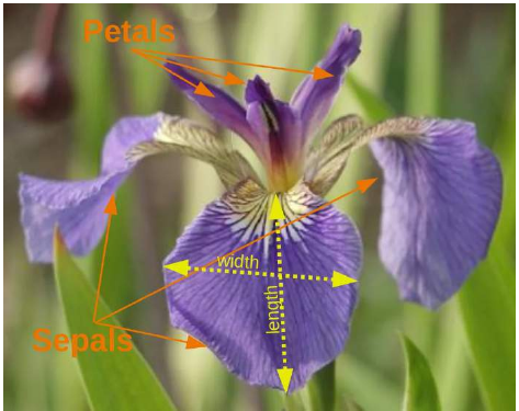
Iris 数据集的特征（Features）：

萼片长度（单位：厘米）

萼片宽度（单位：厘米）

花瓣长度（单位：厘米）

花瓣宽度（单位：厘米）

要预测的目标类别（Target classes）：

鸢尾花-Setosa

鸢尾花-Versicolor

鸢尾花-Virginica

scikit-learn 内嵌了一份 Iris CSV 文件，并提供了一个辅助函数来将其加载到 numpy 数组中：

Python

from sklearn.datasets import load_iris iris = load_iris()

生成的数据集是一个 Bunch 对象：

Python

type(iris)

输出：sklearn.utils.Bunch

您可以使用 keys() 方法查看此数据类型可用的内容：

Python

iris.keys()

输出：dict_keys(['data', 'target', 'target_names', 'DESCR', 'feature_names', 'filename'])

Bunch 对象类似于字典，但它还允许以属性方式访问键：

Python

print(iris["target_names"]) print(iris.target_names)

输出：

['setosa' 'versicolor' 'virginica'] ['setosa' 'versicolor' 'virginica']

每个样本花的特征存储在数据集的 data 属性中：

Python

n_samples, n_features = iris.data.shape print('样本数量:', n_samples) print('特征数量:', n_features) # 第一个样本（第一朵花）的萼片长度、萼片宽度、花瓣长度和花瓣宽度 print(iris.data[0])

输出：

样本数量: 150 特征数量: 4 [5.1 3.5 1.4 0.2]

每朵花的特征都存储在数据集的 data 属性中。让我们看一些样本：

Python

# 索引为 12, 26, 89 和 114 的花 iris.data[[12, 26, 89, 114]]

输出：

array([[4.8, 3. , 1.4, 0.1], [5. , 3.4, 1.6, 0.4], [5.5, 2.5, 4. , 1.3], [5.8, 2.8, 5.1, 2.4]])

关于每个样本类别的信息，即标签，存储在数据集的 target 属性中：

Python

print(iris.data.shape) print(iris.target.shape)

输出：

(150, 4) (150,)

Python

print(iris.target)

输出：

[0 0 0 0 0 0 0 0 0 0 0 0 0 0 0 0 0 0 0 0 0 0 0 0 0 0 0 0 0 0 0 0 0 0 0 0 0 0 0 0 0 0 0 0 0 0 0 0 0 0 1 1 1 1 1 1 1 1 1 1 1 1 1 1 1 1 1 1 1 1 1 1 1 1 1 1 1 1 1 1 1 1 1 1 1 1 1 1 1 1 1 1 1 1 1 1 1 1 1 2 2 2 2 2 2 2 2 2 2 2 2 2 2 2 2 2 2 2 2 2 2 2 2 2 2 2 2 2 2 2 2 2 2 2 2 2 2 2 2 2 2 2 2 2 2 2 2 2 2]

通过使用 NumPy 的 bincount 函数，我们可以看到该数据集中的类别分布均匀——每个物种有 50 朵花：

Python

import numpy as np np.bincount(iris.target)

输出：

array([50, 50, 50])

类别 0： 鸢尾花-Setosa

类别 1： 鸢尾花-Versicolor

类别 2： 鸢尾花-Virginica

这些类别名称存储在最后一个属性，即 target_names 中：

Python

print(iris.target_names)

输出：

['setosa' 'versicolor' 'virginica']

我们 Iris 数据集中每个样本类别的信息存储在数据集的 target 属性中：

Python

print(iris.target)

输出：

[0 0 0 0 0 0 0 0 0 0 0 0 0 0 0 0 0 0 0 0 0 0 0 0 0 0 0 0 0 0 0 0 0 0 0 0 0 0 0 0 0 0 0 0 0 0 0 0 0 0 1 1 1 1 1 1 1 1 1 1 1 1 1 1 1 1 1 1 1 1 1 1 1 1 1 1 1 1 1 1 1 1 1 1 1 1 1 1 1 1 1 1 1 1 1 1 1 1 1 2 2 2 2 2 2 2 2 2 2 2 2 2 2 2 2 2 2 2 2 2 2 2 2 2 2 2 2 2 2 2 2 2 2 2 2 2 2 2 2 2 2 2 2 2 2 2 2 2 2]

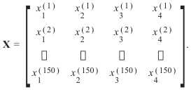
除了数据本身的形状，我们还可以检查标签（即 target.shape）的形状：

每个花样本是数据数组中的一行，列（特征）表示以厘米为单位的花的测量值。例如，我们可以用以下格式表示这个由150个样本和4个特征组成的虹膜数据集，一个二维数组或矩阵r150 × 4：

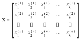
上标表示第i行，下标表示第j个特征。一般来说，我们有n行k列：

Python

print(iris.data.shape) print(iris.target.shape)

输出：

(150, 4) (150,)

NumPy 的 bincount 函数可以计算非负整数数组中每个值的出现次数。我们可以用它来检查数据集中类别的分布：

Python

import numpy as np np.bincount(iris.target)

输出：

array([50, 50, 50])

我们可以看到这些类别是均匀分布的——每个物种有 50 朵花，即：

类别 0： 鸢尾花-Setosa

类别 1： 鸢尾花-Versicolor

类别 2： 鸢尾花-Virginica

这些类别名称存储在最后一个属性，即 target_names 中：

Python

print(iris.target_names)

输出：

['setosa' 'versicolor' 'virginica']

For example, scikit-learn has a very straightforward set of data on these iris species. The data consist of the
following:
• Features in the Iris dataset:
1.
2.
3.
4.
sepal length in cm
sepal width in cm
petal length in cm
petal width in cm
• Target classes to predict:
1.2.3.IrisIrisIrisSetosa
Versicolour
Virginica
scikit-learnarrays:
embeds a copy of the iris CSV file along with a helper function to load it into numpy
18
from sklearn.datasets import load_iris
iris = load_iris()
The resulting dataset is a Bunch object:
type(iris)
Output:sklearn.utils.Bunch
You can see what's available for this data type by using the method keys() :
iris.keys()
Output:dict_keys(['data', 'target', 'target_names', 'DESCR', 'featur
e_names', 'filename'])
A Bunch object is similar to a dicitionary, but it additionally allows accessing the keys in an attribute style:
print(iris["target_names"])
print(iris.target_names)
['setosa' 'versicolor' 'virginica']
['setosa' 'versicolor' 'virginica']
The features of each sample flower are stored in the data attribute of the dataset:
n_samples, n_features = iris.data.shape
print('Number of samples:', n_samples)
print('Number of features:', n_features)
# the sepal length, sepal width, petal length and petal width of t
he first sample (first flower)
print(iris.data[0])
Number of samples: 150
Number of features: 4
[5.1 3.5 1.4 0.2]
The feautures of each flower are stored in the data attribute of the data set. Let's take a look at some of the
samples:
# Flowers with the indices 12, 26, 89, and 114
iris.data[[12, 26, 89, 114]]
19
Output:array([[4.8, 3. , 1.4, 0.1],
[5. , 3.4, 1.6, 0.4],
[5.5, 2.5, 4. , 1.3],
[5.8, 2.8, 5.1, 2.4]])
The information about the class of each sample, i.e. the labels, is stored in the "target" attribute of the data set:
print(iris.data.shape)
print(iris.target.shape)
(150, 4)
(150,)
print(iris.target)
[0 0 0 0 0 0 0 0 0 0 0 0 0 0 0 0 0 0 0 0 0 0 0 0 0 0 0 0 0 0 0 0
0 0 0 0 0
0 0 0 0 0 0 0 0 0 0 0 0 0 1 1 1 1 1 1 1 1 1 1 1 1 1 1 1 1 1 1 1
1 1 1 1 1
1 1 1 1 1 1 1 1 1 1 1 1 1 1 1 1 1 1 1 1 1 1 1 1 1 1 2 2 2 2 2 2
2 2 2 2 2
2 2 2 2 2 2 2 2 2 2 2 2 2 2 2 2 2 2 2 2 2 2 2 2 2 2 2 2 2 2 2 2
2 2 2 2 2
2 2]
import numpy as np
np.bincount(iris.target)
Output:array([50, 50, 50])
Using NumPy's bincount function (above) we can see that the classes in this dataset are evenly distributed -
there are 50 flowers of each species, with
•••class 0: Iris Setosa
class 1: Iris Versicolor
class 2: Iris Virginica
These class names are stored in the last attribute, namely target_names :
print(iris.target_names)
['setosa' 'versicolor' 'virginica']
20
The information about the class of each sample of our Iris dataset is stored in the target attribute of the
dataset:
print(iris.target)
[0 0 0 0 0 0 0 0 0 0 0 0 0 0 0 0 0 0 0 0 0 0 0 0 0 0 0 0 0 0 0 0
0 0 0 0 0
0 0 0 0 0 0 0 0 0 0 0 0 0 1 1 1 1 1 1 1 1 1 1 1 1 1 1 1 1 1 1 1
1 1 1 1 1
1 1 1 1 1 1 1 1 1 1 1 1 1 1 1 1 1 1 1 1 1 1 1 1 1 1 2 2 2 2 2 2
2 2 2 2 2
2 2 2 2 2 2 2 2 2 2 2 2 2 2 2 2 2 2 2 2 2 2 2 2 2 2 2 2 2 2 2 2
2 2 2 2 2
2 2]
Beside of the shape of the data, we can also check the shape of the labels, i.e. the target.shape :
Each flower sample is one row in the data array, and the columns (features) represent the flower measurements
in centimeters. For instance, we can represent this Iris dataset, consisting of 150 samples and 4 features, a
2-dimensional array or matrix R 150 × 4 in the following format:
X =
[
x x x 1
(1
1
150 (2)
(1)
)
xx x 2
(2
2
(1)
(2)
150 )
xx x 3
( 3
3
(1)
150 (2)
)
x x x 4
(4
4
150 (2)
(1)
)
]
.
The superscript denotes the ith row, and the subscript denotes the jth feature, respectively.
Generally, we have n rows and k columns:
X =
[
x x x 1
1
1
(2)
(1)
( n )
x x x2
2
2
(2)
( (1)
n )
x x x 3
3
3
(1)
(2)
( n )
...
...
...
x x x k
k
k
( (2)
(1)
n )
]
.
print(iris.data.shape)
21
print(iris.target.shape)
(150, 4)
(150,)
bincount of NumPy counts the number of occurrences of each value in an array of non-negative integers.
We can use this to check the distribution of the classes in the dataset:
import numpy as np
np.bincount(iris.target)
Output:array([50, 50, 50])
We can see that the classes are distributed uniformly - there are 50 flowers from each species, i.e.
•••class 0: Iris-Setosa
class 1: Iris-Versicolor
class 2: Iris-Virginica
These class names are stored in the last attribute, namely target_names :
print(iris.target_names)
['setosa' 'versicolor' 'virginica']