读取数据并将其转换回“数据”和“标签”(Reading the data and conversion back into 'data' and 'labels')
章节大纲
-
现在我们将演示如何再次读取数据并将其重新分为数据和标签:
Pythonimport numpy as np # 从文件中加载数据 file_data = np.loadtxt("squirrels.txt") # 分离数据(所有列,除了最后一列) data = file_data[:, :-1] # 分离标签(最后一列) labels = file_data[:, 2:] # 将标签从二维列向量重新形状为一维数组 labels = labels.reshape((labels.shape[0]))我们将数据文件命名为
squirrels.txt,因为我们想象着一种生活在撒哈拉沙漠中的奇特动物。X 值代表这些动物的夜视能力,Y 值对应着毛皮的颜色,从沙色到黑色。我们有三种松鼠:0、1 和 2。(请注意,我们的松鼠是虚构的,与撒哈拉沙漠中真实的松鼠无关!)Pythonimport matplotlib.pyplot as plt colours = ('green', 'red', 'blue', 'magenta', 'yellow', 'cyan') n_classes = 3 # 类别数量 fig, ax = plt.subplots() # 遍历每个类别并绘制散点图 for n_class in range(0, n_classes): ax.scatter(data[labels==n_class, 0], data[labels==n_class, 1], c=colours[n_class], s=10, label=str(n_class)) ax.set(xlabel='夜视能力', ylabel='毛色 (沙色到黑色, 0到10)', title='撒哈拉虚拟松鼠') ax.legend(loc='upper right') plt.show()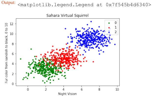
训练人工数据
在下面的代码中,我们将训练我们的人工数据:
Pythonfrom sklearn.model_selection import train_test_split from sklearn.neighbors import KNeighborsClassifier from sklearn import metrics # 将数据分为训练集和测试集 data_sets = train_test_split(data, labels, train_size=0.8, # 训练集比例 test_size=0.2, # 测试集比例 random_state=42 # 随机种子,保证每次运行结果一致 ) train_data, test_data, train_labels, test_labels = data_sets # 导入模型 (K近邻分类器) # from sklearn.neighbors import KNeighborsClassifier # 已经在上面导入 # 创建分类器实例,设置 K 值为 8 knn = KNeighborsClassifier(n_neighbors=8) # 训练模型 knn.fit(train_data, train_labels) # 在测试集上进行预测 calculated_labels = knn.predict(test_data) print(calculated_labels)输出:
array([2., 0., 1., 1., 0., 1., 2., 2., 2., 2., 0., 1., 0., 0., 1., 0., 1., 2., 0., 0., 1., 2., 1., 2., 2., 1., 2., 0., 0., 2., 0., 2., 2., 0., 0., 2., 0., 0., 0., 1., 0., 1., 1., 2., 0., 2., 1., 2., 1., 0., 2., 1., 1., 0., 1., 2., 1., 0., 0., 2., 1., 0., 1., 1., 0., 0., 0., 0., 0., 0., 0., 1., 1., 0., 1., 1., 1., 0., 1., 2., 1., 2., 0., 2., 1., 1., 0., 2., 2., 2., 0., 1., 1., 1., 2., 2., 0., 2., 2., 2., 2., 0., 0., 1., 1., 1., 2., 1., 1., 1., 0., 2., 1., 2., 0., 0., 1., 0., 1., 0., 2., 2., 2., 1., 1., 1., 0., 2., 1., 2., 2., 1., 2., 0., 2., 0., 0., 1., 0., 2., 2., 0., 0., 1., 2., 1., 2., 0., 0., 2., 2., 0., 0., 1., 2., 1., 2., 0., 0., 1., 2., 1., 0., 2., 2., 0., 2., 0., 0., 2., 1., 0., 0., 0., 0., 2., 2., 1., 0., 2., 2., 1., 2., 0., 1., 1., 1., 0., 1., 0., 1., 1., 2., 0., 2., 2., 1., 1., 1., 2.])Python# 导入 metrics (评估指标) # from sklearn import metrics # 已经在上面导入 # 计算准确率 print("准确率:", metrics.accuracy_score(test_labels, calculated_labels))输出:
准确率: 0.97
We will demonstrate now, how to read in the data again and how to split it into data and labels again:
file_data = np.loadtxt("squirrels.txt")
data = file_data[:,:-1]
labels = file_data[:,2:]
labels = labels.reshape((labels.shape[0]))
We had called the data file squirrels.txt , because we imagined a strange kind of animal living in the
Sahara desert. The x-values stand for the night vision capabilities of the animals and the y-values correspond
to the colour of the fur, going from sandish to black. We have three kinds of squirrels, 0, 1, and 2. (Be aware
that our squirrals are imaginary squirrels and have nothing to do with the real squirrels of the Sahara!)
import matplotlib.pyplot as plt
colours = ('green', 'red', 'blue', 'magenta', 'yellow', 'cyan')
n_classes = 3
fig, ax = plt.subplots()
for n_class in range(0, n_classes):
ax.scatter(data[labels==n_class, 0], data[labels==n_class,
1],
c=colours[n_class], s=10, label=str(n_class))
ax.set(xlabel='Night Vision',
ylabel='Fur color from sandish to black, 0 to 10 ',
title='Sahara Virtual Squirrel')
ax.legend(loc='upper right')
51
Output:<matplotlib.legend.Legend at 0x7f545b4d6340>
We will train our articifical data in the following code:
from sklearn.model_selection import train_test_split
data_sets = train_test_split(data,
labels,
train_size=0.8,
test_size=0.2,
random_state=42 # garantees same output fo
r every run
)
train_data, test_data, train_labels, test_labels = data_sets
# import model
from sklearn.neighbors import KNeighborsClassifier
# create classifier
knn = KNeighborsClassifier(n_neighbors=8)
# train
knn.fit(train_data,train_labels)
# test on test data:
calculated_labels = knn.predict(test_data)
calculated_labels
52
Output:array([2., 0., 1., 1., 0., 1., 2., 2., 2., 2., 0., 1., 0.,
0., 1., 0., 1.,
2., 0., 0., 1., 2., 1., 2., 2., 1., 2., 0., 0., 2.,
0., 2., 2., 0.,
0., 2., 0., 0., 0., 1., 0., 1., 1., 2., 0., 2., 1.,
2., 1., 0., 2.,
1., 1., 0., 1., 2., 1., 0., 0., 2., 1., 0., 1., 1.,
0., 0., 0., 0.,
0., 0., 0., 1., 1., 0., 1., 1., 1., 0., 1., 2., 1.,
2., 0., 2., 1.,
1., 0., 2., 2., 2., 0., 1., 1., 1., 2., 2., 0., 2.,
2., 2., 2., 0.,
0., 1., 1., 1., 2., 1., 1., 1., 0., 2., 1., 2., 0.,
0., 1., 0., 1.,
0., 2., 2., 2., 1., 1., 1., 0., 2., 1., 2., 2., 1.,
2., 0., 2., 0.,
0., 1., 0., 2., 2., 0., 0., 1., 2., 1., 2., 0., 0.,
2., 2., 0., 0.,
1., 2., 1., 2., 0., 0., 1., 2., 1., 0., 2., 2., 0.,
2., 0., 0., 2.,
1., 0., 0., 0., 0., 2., 2., 1., 0., 2., 2., 1., 2.,
0., 1., 1., 1.,
0., 1., 0., 1., 1., 2., 0., 2., 2., 1., 1., 1., 2.])
from sklearn import metrics
print("Accuracy:", metrics.accuracy_score(test_labels, calculate
d_labels))
Accuracy: 0.97