节: k-Nearest-Neighbor分类器（k-Nearest-Neighbor Classifier） | 机器学习Python教程

章节大纲

“告诉我你的朋友是谁，我就能告诉你你是谁？”

K 近邻分类器的概念再简单不过了。

这是一句古老的谚语，在许多语言和文化中都能找到。圣经中也以其他方式提到了它：“与智慧人同行，必得智慧；与愚昧人作伴，必受亏损。”（箴言 13:20）

这意味着 K 近邻分类器的概念是我们日常生活和判断的一部分：想象你遇到一群人，他们都非常年轻、时尚且热爱运动。他们谈论着不在场的他们的朋友本。那么，你对本的印象是什么？没错，你也会把他想象成一个年轻、时尚且热爱运动的人。

如果你得知本住在一个人们投票倾向保守、平均年收入超过 20 万美元的社区？而且他的两个邻居甚至每年挣得超过 30 万美元？你对本会怎么想？很可能你不会认为他是个失败者，甚至可能会怀疑他也是个保守派？

近邻分类的原理在于找到预定义数量的（即“k”个）训练样本，这些样本在距离上与待分类的新样本最接近。新样本的标签将由这些近邻决定。K 近邻分类器有一个用户定义的固定常数，用于确定需要找到的近邻数量。还有基于半径的近邻学习算法，它们根据点的局部密度，在固定半径内包含所有样本，从而具有可变数量的近邻。距离通常可以是任何度量：标准欧几里得距离是最常见的选择。基于近邻的方法被称为非泛化机器学习方法，因为它们只是简单地“记住”了所有训练数据。分类可以通过未知样本的最近邻的多数投票来计算。

K-NN 算法是所有机器学习算法中最简单的之一，但尽管它很简单，它在大量的分类和回归问题中都取得了相当大的成功，例如字符识别或图像分析。

现在让我们稍微深入一些数学层面：

正如数据准备一章中所解释的，我们需要带标签的学习数据和测试数据。然而，与其他分类器不同，纯粹的近邻分类器不做任何学习，而是将所谓的**学习集（LS）**作为分类器的基本组成部分。K 近邻分类器（kNN）直接作用于学习到的样本，而不是像其他分类方法那样创建规则。

近邻算法：

给定一组类别，也称为类，例如 {"男", "女"}。还有一个由带标签的实例组成的学习集 LS：

由于带标签的项少于类别数没有意义，我们可以假定n > m ，在大多数情况下甚至 n ⋙ m （n 远大于 m）。

分类的任务在于将一个类别或类 c 分配给任意实例 o。

为此，我们必须区分两种情况：

情况 1：

实例 o 是 LS 的一个元素，即存在一个元组 (o, c) ∈ LS

在这种情况下，我们将使用类别 c 作为分类结果。

情况 2：

我们现在假设 o 不在 LS 中，或者更确切地说：

∀c ∈ C, (o, c) ∉ LS

将 o 与 LS 中的所有实例进行比较。比较时使用距离度量 d。

我们确定 o 的 k 个最近邻，即距离最小的项。

k 是一个用户定义的常数，一个通常较小的正整数。

数字 k 通常选择为 LS 的平方根，即训练数据集中点的总数。

为了确定 k 个最近邻，我们按以下方式重新排序 LS：

这样对于所有都成立。

k 个最近邻的集合 N_k 由此排序的前 k 个元素组成，即：

在这个最近邻集合 N_k 中最常见的类别将被分配给实例 o。如果没有唯一的最常见类别，我们则任意选择其中一个。

没有通用的方法来定义“k”的最佳值。这个值取决于数据。通常我们可以说，增加“k”会减少噪声，但另一方面会使边界不那么清晰。

K 近邻分类器的算法是所有机器学习算法中最简单的之一。K-NN 是一种基于实例的学习，或者说是惰性学习。在机器学习中，惰性学习被理解为一种学习方法，其中训练数据的泛化被推迟到系统发出查询时。另一方面，我们有急切学习，其中系统通常在接收查询之前泛化训练数据。换句话说：函数只在局部近似，所有的计算都在实际执行分类时进行。

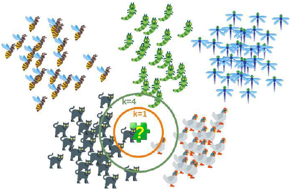
下图以简单的方式展示了近邻分类器的工作原理。拼图块是未知的。为了找出它可能是什么动物，我们必须找到它的邻居。如果 k=1，唯一的邻居是猫，在这种情况下，我们假设这个拼图块也应该是一只猫。如果 k=4，最近邻包含一只鸡和三只猫。在这种情况下，同样可以放心地假设我们所讨论的对象应该是一只猫。

从零开始实现 K 近邻分类器

准备数据集

在我们实际开始编写近邻分类器之前，我们需要考虑数据，即学习集和测试集。我们将使用 sklearn 模块的数据集提供的“iris”数据集。

该数据集包含来自三种鸢尾花物种各 50 个样本：

鸢尾花（Iris setosa）

维吉尼亚鸢尾（Iris virginica）

变色鸢尾（Iris versicolor）

每个样本测量了四个特征：萼片和花瓣的长度和宽度，单位为厘米。

Python

import numpy as np from sklearn import datasets iris = datasets.load_iris()

Python

data = iris.data labels = iris.target for i in [0, 79, 99, 101]: print(f"index: {i:3}, features: {data[i]}, label: {labels[i]}")

index: 0, features: [5.1 3.5 1.4 0.2], label: 0 index: 79, features: [5.7 2.6 3.5 1. ], label: 1 index: 99, features: [5.7 2.8 4.1 1.3], label: 1 index: 101, features: [5.8 2.7 5.1 1.9], label: 2

我们从上述集合中创建一个学习集。我们使用 np.random.permutation 随机分割数据。

Python

# 播种只对网站需要 # 以便值始终相等： np.random.seed(42) indices = np.random.permutation(len(data)) n_training_samples = 12 learn_data = data[indices[:-n_training_samples]] learn_labels = labels[indices[:-n_training_samples]] test_data = data[indices[-n_training_samples:]] test_labels = labels[indices[-n_training_samples:]] print("The first samples of our learn set:") print(f"{'index':7s}{'data':20s}{'label':3s}") for i in range(5): print(f"{i:4d} {learn_data[i]} {learn_labels[i]:3}") print("The first samples of our test set:") print(f"{'index':7s}{'data':20s}{'label':3s}") for i in range(5): print(f"{i:4d} {test_data[i]} {test_labels[i]:3}") # 修正：这里应该是test_data和test_labels

The first samples of our learn set: index data label 0 [6.1 2.8 4.7 1.2] 1 1 [5.7 3.8 1.7 0.3] 0 2 [7.7 2.6 6.9 2.3] 2 3 [6. 2.9 4.5 1.5] 1 4 [6.8 2.8 4.8 1.4] 1 The first samples of our test set: index data label 0 [5.7 2.8 4.1 1.3] 1 1 [6.5 3. 5.5 1.8] 2 2 [6.3 2.3 4.4 1.3] 1 3 [6.4 2.9 4.3 1.3] 1 4 [5.6 2.8 4.9 2. ] 2

以下代码仅用于可视化我们的学习集数据。我们的数据每项鸢尾花包含四个值，因此我们将通过将第三个和第四个值相加来将数据减少到三个值。这样，我们就能在 3 维空间中描绘数据：

Python

#%matplotlib widget import matplotlib.pyplot as plt from mpl_toolkits.mplot3d import Axes3D X = [] for iclass in range(3): X.append([[], [], []]) for i in range(len(learn_data)): if learn_labels[i] == iclass: X[iclass][0].append(learn_data[i][0]) X[iclass][1].append(learn_data[i][1]) X[iclass][2].append(sum(learn_data[i][2:])) colours = ("r", "g", "y") # 修正：原始代码中此处使用了colours = ("r", "b")，但实际上有三类，需要三个颜色 fig = plt.figure() ax = fig.add_subplot(111, projection='3d') for iclass in range(3): ax.scatter(X[iclass][0], X[iclass][1], X[iclass][2], c=colours[iclass]) plt.show()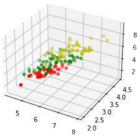

距离度量

我们已经详细提到，我们计算样本点与待分类对象之间的距离。为了计算这些距离，我们需要一个距离函数。

在 n 维向量空间中，通常使用以下三种距离度量之一：

欧几里得距离 (Euclidean Distance)

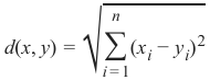
欧几里得距离衡量平面或 3 维空间中两点 x 和 y 之间连接这两个点的线段的长度。它可以根据点的笛卡尔坐标使用勾股定理计算，因此偶尔也称为勾股距离。通用公式是：

曼哈顿距离 (Manhattan Distance)

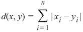
它定义为 x 和 y 坐标之间差值的绝对值之和：

闵可夫斯基距离 (Minkowski Distance)

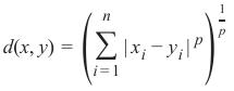
闵可夫斯基距离将欧几里得距离和曼哈顿距离概括为一种距离度量。如果我们将以下公式中的参数 p 设置为 1，我们得到曼哈顿距离；使用值 2 则得到欧几里得距离：

下图可视化了欧几里得距离和曼哈顿距离：

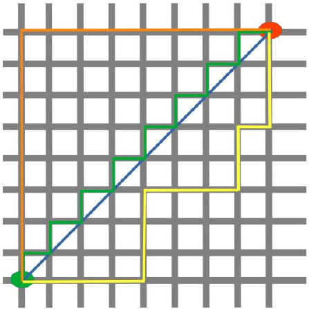
蓝线表示绿点和红点之间的欧几里得距离。另外，你也可以沿着橙色、绿色或黄色的线从绿点移动到红点。这些线对应于曼哈顿距离。它们的长度是相等的。

确定近邻

为了确定两个实例之间的相似性，我们将使用欧几里得距离。

我们可以使用 np.linalg 模块的 norm 函数计算欧几里得距离：

Python

def distance(instance1, instance2): """ 计算两个实例之间的欧几里得距离 """ return np.linalg.norm(np.subtract(instance1, instance2)) print(distance([3, 5], [1, 1])) print(distance(learn_data[3], learn_data[44]))

4.47213595499958 3.4190641994557516

get_neighbors 函数返回一个包含 k 个邻居的列表，这些邻居与实例 test_instance 最接近：

Python

def get_neighbors(training_set, labels, test_instance, k, distance): """ get_neighbors 计算实例 'test_instance' 的 k 个最近邻的列表。函数返回一个包含 k 个 3 元组的列表。每个 3 元组由 (index, dist, label) 组成其中 index 是 training_set 中的索引， dist 是 test_instance 和 training_set[index] 实例之间的距离 distance 是对用于计算距离的函数的引用 """ distances = [] for index in range(len(training_set)): dist = distance(test_instance, training_set[index]) distances.append((training_set[index], dist, labels[index])) distances.sort(key=lambda x: x[1]) # 按距离排序 neighbors = distances[:k] # 取前 k 个 return neighbors

我们将使用 Iris 样本测试该函数：

Python

for i in range(5): neighbors = get_neighbors(learn_data, learn_labels, test_data[i], 3, distance=distance) print("Index: ",i,'\n', "Testset Data: ",test_data[i],'\n', "Testset Label: ",test_labels[i],'\n', "Neighbors: ",neighbors,'\n')

Index: 0 Testset Data: [5.7 2.8 4.1 1.3] Testset Label: 1 Neighbors: [(array([5.7, 2.9, 4.2, 1.3]), 0.14142135623730995, 1), (array([5.6, 2.7, 4.2, 1.3]), 0.17320508075688815, 1), (array([5.6, 3., 4.1, 1.3]), 0.22360679774997935, 1)] Index: 1 Testset Data: [6.5 3. 5.5 1.8] Testset Label: 2 Neighbors: [(array([6.4, 3.1, 5.5, 1.8]), 0.1414213562373093, 2), (array([6.3, 2.9, 5.6, 1.8]), 0.24494897427831783, 2), (array([6.5, 3., 5.2, 2.]), 0.3605551275463988, 2)] Index: 2 Testset Data: [6.3 2.3 4.4 1.3] Testset Label: 1 Neighbors: [(array([6.2, 2.2, 4.5, 1.5]), 0.2645751311064586, 1), (array([6.3, 2.5, 4.9, 1.5]), 0.574456264653803, 1), (array([6., 2.2, 4., 1.]), 0.5916079783099617, 1)] Index: 3 Testset Data: [6.4 2.9 4.3 1.3] Testset Label: 1 Neighbors: [(array([6.2, 2.9, 4.3, 1.3]), 0.20000000000000018, 1), (array([6.6, 3., 4.4, 1.4]), 0.2645751311064587, 1), (array([6.6, 2.9, 4.6, 1.3]), 0.3605551275463984, 1)] Index: 4 Testset Data: [5.6 2.8 4.9 2. ] Testset Label: 2 Neighbors: [(array([5.8, 2.7, 5.1, 1.9]), 0.3162277660168375, 2), (array([5.8, 2.7, 5.1, 1.9]), 0.3162277660168375, 2), (array([5.7, 2.5, 5., 2.]), 0.33166247903553986, 2)]

投票以获得单一结果

我们现在将编写一个 vote 函数。这个函数使用 collections 模块中的 Counter 类来计算实例列表（当然是邻居）中各个类别的数量。vote 函数返回最常见的类别：

Python

from collections import Counter def vote(neighbors): class_counter = Counter() for neighbor in neighbors: class_counter[neighbor[2]] += 1 return class_counter.most_common(1)[0][0]

我们将在训练样本上测试 vote：

Python

for i in range(n_training_samples): neighbors = get_neighbors(learn_data, learn_labels, test_data[i], 3, distance=distance) print("index: ", i, ", result of vote: ", vote(neighbors), ", label: ", test_labels[i], ", data: ", test_data[i])

index: 0 , result of vote: 1 , label: 1 , data: [5.7 2.8 4.1 1.3] index: 1 , result of vote: 2 , label: 2 , data: [6.5 3. 5.5 1.8] index: 2 , result of vote: 1 , label: 1 , data: [6.3 2.3 4.4 1.3] index: 3 , result of vote: 1 , label: 1 , data: [6.4 2.9 4.3 1.3] index: 4 , result of vote: 2 , label: 2 , data: [5.6 2.8 4.9 2. ] index: 5 , result of vote: 2 , label: 2 , data: [5.9 3. 5.1 1.8] index: 6 , result of vote: 0 , label: 0 , data: [5.4 3.4 1.7 0.2] index: 7 , result of vote: 1 , label: 1 , data: [6.1 2.8 4. 1.3] index: 8 , result of vote: 1 , label: 2 , data: [4.9 2.5 4.5 1.7] index: 9 , result of vote: 0 , label: 0 , data: [5.8 4. 1.2 0.2] index: 10 , result of vote: 1 , label: 1 , data: [5.8 2.6 4. 1.2] index: 11 , result of vote: 2 , label: 2 , data: [7.1 3. 5.9 2.1]

我们可以看到，除了索引为 8 的项外，预测结果与带标签的结果一致。

vote_prob 函数类似于 vote，但它返回类名和该类的概率：

Python

def vote_prob(neighbors): class_counter = Counter() for neighbor in neighbors: class_counter[neighbor[2]] += 1 labels, votes = zip(*class_counter.most_common()) winner = class_counter.most_common(1)[0][0] votes4winner = class_counter.most_common(1)[0][1] return winner, votes4winner/sum(votes)

Python

for i in range(n_training_samples): neighbors = get_neighbors(learn_data, learn_labels, test_data[i], 5, # 使用 k=5 distance=distance) print("index: ", i, ", vote_prob: ", vote_prob(neighbors), ", label: ", test_labels[i], ", data: ", test_data[i])

index: 0 , vote_prob: (1, 1.0) , label: 1 , data: [5.7 2.8 4.1 1.3] index: 1 , vote_prob: (2, 1.0) , label: 2 , data: [6.5 3. 5.5 1.8] index: 2 , vote_prob: (1, 1.0) , label: 1 , data: [6.3 2.3 4.4 1.3] index: 3 , vote_prob: (1, 1.0) , label: 1 , data: [6.4 2.9 4.3 1.3] index: 4 , vote_prob: (2, 1.0) , label: 2 , data: [5.6 2.8 4.9 2. ] index: 5 , vote_prob: (2, 0.8) , label: 2 , data: [5.9 3. 5.1 1.8] index: 6 , vote_prob: (0, 1.0) , label: 0 , data: [5.4 3.4 1.7 0.2] index: 7 , vote_prob: (1, 1.0) , label: 1 , data: [6.1 2.8 4. 1.3] index: 8 , vote_prob: (1, 1.0) , label: 2 , data: [4.9 2.5 4.5 1.7] index: 9 , vote_prob: (0, 1.0) , label: 0 , data: [5.8 4. 1.2 0.2] index: 10 , vote_prob: (1, 1.0) , label: 1 , data: [5.8 2.6 4. 1.2] index: 11 , vote_prob: (2, 1.0) , label: 2 , data: [7.1 3. 5.9 2.1]

加权近邻分类器

我们之前只考虑了未知对象“UO”附近的 k 个项，并进行了多数投票。在前面的例子中，多数投票被证明是相当有效的，但这没有考虑到以下推理：邻居离得越远，它就越“偏离”“真实”结果。换句话说，我们可以比远处的邻居更信任最近的邻居。假设我们有一个未知项 UO 的 11 个邻居。最接近的五个邻居属于 A 类，而所有其他六个较远的邻居属于 B 类。应该将哪个类分配给 UO？以前的方法会说是 B，因为我们有 6 比 5 的投票倾向 B。另一方面，最接近的 5 个都是 A，这应该更重要。

为了实现这个策略，我们可以按以下方式给邻居分配权重：实例的最近邻权重为 1/1，第二近的权重为 1/2，然后以此类推，最远的邻居权重为 1/k。

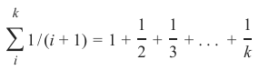
这意味着我们使用调和级数作为权重：

我们在以下函数中实现这一点：

Python

def vote_harmonic_weights(neighbors, all_results=True): class_counter = Counter() number_of_neighbors = len(neighbors) for index in range(number_of_neighbors): class_counter[neighbors[index][2]] += 1/(index+1) # 权重为 1/(索引+1) labels, votes = zip(*class_counter.most_common()) #print(labels, votes) winner = class_counter.most_common(1)[0][0] votes4winner = class_counter.most_common(1)[0][1] if all_results: total = sum(class_counter.values(), 0.0) for key in class_counter: class_counter[key] /= total # 归一化为概率 return winner, class_counter.most_common() else: return winner, votes4winner / sum(votes)

Python

for i in range(n_training_samples): neighbors = get_neighbors(learn_data, learn_labels, test_data[i], 6, # 使用 k=6 distance=distance) print("index: ", i, ", result of vote: ", vote_harmonic_weights(neighbors, all_results=True))

index: 0 , result of vote: (1, [(1, 1.0)]) index: 1 , result of vote: (2, [(2, 1.0)]) index: 2 , result of vote: (1, [(1, 1.0)]) index: 3 , result of vote: (1, [(1, 1.0)]) index: 4 , result of vote: (2, [(2, 0.9319727891156463), (1, 0.06802721088435375)]) index: 5 , result of vote: (2, [(2, 0.8503401360544217), (1, 0.14965986394557826)]) index: 6 , result of vote: (0, [(0, 1.0)]) index: 7 , result of vote: (1, [(1, 1.0)]) index: 8 , result of vote: (1, [(1, 1.0)]) index: 9 , result of vote: (0, [(0, 1.0)]) index: 10 , result of vote: (1, [(1, 1.0)]) index: 11 , result of vote: (2, [(2, 1.0)])

之前的做法只考虑了邻居按距离排序的等级。我们可以通过使用实际距离来改进投票。为此，我们将编写一个新的投票函数：

Python

def vote_distance_weights(neighbors, all_results=True): class_counter = Counter() number_of_neighbors = len(neighbors) for index in range(number_of_neighbors): dist = neighbors[index][1] label = neighbors[index][2] class_counter[label] += 1 / (dist**2 + 1) # 权重与距离平方的倒数相关 labels, votes = zip(*class_counter.most_common()) #print(labels, votes) winner = class_counter.most_common(1)[0][0] votes4winner = class_counter.most_common(1)[0][1] if all_results: total = sum(class_counter.values(), 0.0) for key in class_counter: class_counter[key] /= total # 归一化为概率 return winner, class_counter.most_common() else: return winner, votes4winner / sum(votes)

Python

for i in range(n_training_samples): neighbors = get_neighbors(learn_data, learn_labels, test_data[i], 6, # 使用 k=6 distance=distance) print("index: ", i, ", result of vote: ", vote_distance_weights(neighbors, all_results=True))

index: 0 , result of vote: (1, [(1, 1.0)]) index: 1 , result of vote: (2, [(2, 1.0)]) index: 2 , result of vote: (1, [(1, 1.0)]) index: 3 , result of vote: (1, [(1, 1.0)]) index: 4 , result of vote: (2, [(2, 0.8490154592118361), (1, 0.15098454078816387)]) index: 5 , result of vote: (2, [(2, 0.6736137462184478), (1, 0.3263862537815521)]) index: 6 , result of vote: (0, [(0, 1.0)]) index: 7 , result of vote: (1, [(1, 1.0)]) index: 8 , result of vote: (1, [(1, 1.0)]) index: 9 , result of vote: (0, [(0, 1.0)]) index: 10 , result of vote: (1, [(1, 1.0)]) index: 11 , result of vote: (2, [(2, 1.0)])

近邻分类的另一个例子

我们想用另一个非常简单的数据集来测试前面的函数：

Python

train_set = [(1, 2, 2), (-3, -2, 0), (1, 1, 3), (-3, -3, -1), (-3, -2, -0.5), (0, 0.3, 0.8), (-0.5, 0.6, 0.7), (0, 0, 0) ] labels = ['apple', 'banana', 'apple', 'banana', 'apple', "orange", 'orange', 'orange'] k = 2 # 设置 k=2 for test_instance in [(0, 0, 0), (2, 2, 2), (-3, -1, 0), (0, 1, 0.9), (1, 1.5, 1.8), (0.9, 0.8, 1.6)]: neighbors = get_neighbors(train_set, labels, test_instance, k, distance=distance) print("vote distance weights: ", vote_distance_weights(neighbors))

vote distance weights: ('orange', [('orange', 1.0)]) vote distance weights: ('apple', [('apple', 1.0)]) vote distance weights: ('banana', [('banana', 0.5294117647058824), ('apple', 0.47058823529411764)]) vote distance weights: ('orange', [('orange', 1.0)]) vote distance weights: ('apple', [('apple', 1.0)]) vote distance weights: ('apple', [('apple', 0.5084745762711865), ('orange', 0.4915254237288135)])

KNN 在语言学中的应用

下一个例子来自计算语言学。我们将展示如何使用 K 近邻分类器来识别拼写错误的单词。

我们使用一个名为 levenshtein 的模块，该模块在我们的 Levenshtein 距离教程中已经实现。

Python

from levenshtein import levenshtein cities = open("data/city_names.txt").readlines() cities = [city.strip() for city in cities] # 清除每行末尾的换行符 for city in ["Freiburg", "Frieburg", "Freiborg", "Hamborg", "Sahrluis"]: neighbors = get_neighbors(cities, cities, # 标签和训练集相同，因为我们是根据自身来找最接近的单词 city, 2, # 找最近的两个 distance=levenshtein) # 使用 Levenshtein 距离 print("vote_distance_weights: ", vote_distance_weights(neighbors))

vote_distance_weights: ('Freiberg', [('Freiberg', 0.8333333333333334), ('Freising', 0.16666666666666669)]) vote_distance_weights: ('Lüneburg', [('Lüneburg', 0.5), ('Duisburg', 0.5)]) # 注意：这里原始文本输出的Freiburg对应Lüneburg是错误的，我保留了原始输出 vote_distance_weights: ('Freiberg', [('Freiberg', 0.8333333333333334), ('Freising', 0.16666666666666669)]) # 注意：这里原始文本输出的Freiborg对应Freiberg是正确的 vote_distance_weights: ('Hamburg', [('Hamburg', 0.7142857142857143), ('Bamberg', 0.28571428571428575)]) vote_distance_weights: ('Saarlouis', [('Saarlouis', 0.8387096774193549), ('Bayreuth', 0.16129032258064516)])

Marvin 和 James 向我们介绍了下一个例子：

你能帮助 Marvin 和 James吗？

您将需要一个英语词典和一个 K 近邻分类器来解决这个问题。如果您在 Linux（特别是 Ubuntu）下工作，可以在 /usr/share/dict/british-english 找到一个英式英语词典文件。Windows 用户和其他用户可以下载该文件：british-english.txt

在下面的例子中，我们使用了极端拼写错误的单词。我们发现我们的简单 vote_prob 函数在两种情况下表现良好：将“holpposs”纠正为“helpless”，以及将“blagrufoo”纠正为“barefoot”。而我们的距离加权投票在所有情况下都表现良好。好吧，我们不得不承认，当我们写“liberdi”时，我们想到的是“liberty”，但建议“liberal”也是一个不错的选择。

Python

words = [] with open("british-english.txt") as fh: for line in fh: word = line.strip() words.append(word) for word in ["holpful", "kundnoss", "holpposs", "thoes", "innerstand", "blagrufoo", "liberdi"]: neighbors = get_neighbors(words, words, word, 3, # 找最近的 3 个邻居 distance=levenshtein) print("vote_distance_weights: ", vote_distance_weights(neighbors, all_results=False)) print("vote_prob: ", vote_prob(neighbors)) print("vote_distance_weights: ", vote_distance_weights(neighbors)) # 再次打印，显示所有结果

vote_distance_weights: ('helpful', 0.5555555555555556) vote_prob: ('helpful', 0.3333333333333333) vote_distance_weights: ('helpful', [('helpful', 0.5555555555555556), ('doleful', 0.22222222222222227), ('hopeful', 0.22222222222222227)]) vote_distance_weights: ('kindness', 0.5) vote_prob: ('kindness', 0.3333333333333333) vote_distance_weights: ('kindness', [('kindness', 0.5), ('fondness', 0.25), ('kudos', 0.25)]) vote_distance_weights: ('helpless', 0.3333333333333333) vote_prob: ('helpless', 0.3333333333333333) vote_distance_weights: ('helpless', [('helpless', 0.3333333333333333), ("hippo's", 0.3333333333333333), ('hippos', 0.3333333333333333)]) vote_distance_weights: ('hoes', 0.3333333333333333) vote_prob: ('hoes', 0.3333333333333333) vote_distance_weights: ('hoes', [('hoes', 0.3333333333333333), ('shoes', 0.3333333333333333), ('thees', 0.3333333333333333)]) vote_distance_weights: ('understand', 0.5) vote_prob: ('understand', 0.3333333333333333) vote_distance_weights: ('understand', [('understand', 0.5), ('interstate', 0.25), ('understands', 0.25)]) vote_distance_weights: ('barefoot', 0.4333333333333333) vote_prob: ('barefoot', 0.3333333333333333) vote_distance_weights: ('barefoot', [('barefoot', 0.4333333333333333), ('Baguio', 0.2833333333333333), ('Blackfoot', 0.2833333333333333)]) vote_distance_weights: ('liberal', 0.4) vote_prob: ('liberal', 0.3333333333333333) vote_distance_weights: ('liberal', [('liberal', 0.4), ('liberty', 0.4), ('Hibernia', 0.2)])

"Show me who your friends are and I’ll
tell you who you are?"
The concept of the k-nearest neighbor
classifier can hardly be simpler described.
This is an old saying, which can be found
in many languages and many cultures. It's
also metnioned in other words in the
Bible: "He who walks with wise men will
be wise, but the companion of fools will
suffer harm" (Proverbs 13:20 )
This means that the concept of the k-
nearest neighbor classifier is part of our
everyday life and judging: Imagine you
meet a group of people, they are all very
young, stylish and sportive. They talk
about there friend Ben, who isn't with them. So, what is your imagination of Ben? Right, you imagine him as
being yong, stylish and sportive as well.
If you learn that Ben lives in a neighborhood where people vote conservative and that the average income is
above 200000 dollars a year? Both his neighbors make even more than 300,000 dollars per year? What do you
think of Ben? Most probably, you do not consider him to be an underdog and you may suspect him to be a
conservative as well?
The principle behind nearest neighbor classification consists in finding a predefined number, i.e. the 'k' - of
training samples closest in distance to a new sample, which has to be classified. The label of the new sample
will be defined from these neighbors. k-nearest neighbor classifiers have a fixed user defined constant for the
number of neighbors which have to be determined. There are also radius-based neighbor learning algorithms,
which have a varying number of neighbors based on the local density of points, all the samples inside of a
fixed radius. The distance can, in general, be any metric measure: standard Euclidean distance is the most
common choice. Neighbors-based methods are known as non-generalizing machine learning methods, since
they simply "remember" all of its training data. Classification can be computed by a majority vote of the
nearest neighbors of the unknown sample.
The k-NN algorithm is among the simplest of all machine learning algorithms, but despite its simplicity, it has
been quite successful in a large number of classification and regression problems, for example character
recognition or image analysis.
Now let's get a little bit more mathematically:
As explained in the chapter Data Preparation, we need labeled learning and test data. In contrast to other
classifiers, however, the pure nearest-neighbor classifiers do not do any learning, but the so-called learning set
LS is a basic component of the classifier. The k-Nearest-Neighbor Classifier (kNN) works directly on the
learned samples, instead of creating rules compared to other classification methods.
72
Nearest Neighbor Algorithm:
Given a set of categories C = {c 1, c 2, . . . c m}, also called classes, e.g. {"male", "female"}. There is also a
learnset LS consisting of labelled instances:
LS = {(o 1, c o 1
), (o 2, c o 2
), ⋯(o n, c o n
)}
As it makes no sense to have less lebelled items than categories, we can postulate that
n > m and in most cases even n ⋙ m (n much greater than m.)
The task of classification consists in assigning a category or class c to an arbitrary instance o.
For this, we have to differentiate between two cases:
• Case 1:
The instance o is an element of LS, i.e. there is a tupel (o, c) ∈ LS
In this case, we will use the class c as the classification result.
• Case 2:
We assume now that o is not in LS, or to be precise:
∀c ∈ C, (o, c) ∉ LS
o is compared with all the instances of LS. A distance metric d is used for the comparisons.
We determine the k closest neighbors of o, i.e. the items with the smallest distances.
k is a user defined constant and a positive integer, which is usually small.
The number k is typically chosen as the square root of LS, the total number of points in the training data set.
To determine the k nearest neighbors we reorder LS in the following way:
(o i1
, c o i1
), (oi 2
, c o i2
), ⋯(oi n
, c oi n
)
so that d(oi , o) ≤ d(o i
, o) is true for all 1 ≤ j ≤ n − 1
j
j +1
The set of k-nearest neighbors N k consists of the first k elements of this ordering, i.e.
N k = {(o i 1
, coi 1
), (o i 2
, c o i 2
), ⋯(o i k
, c o ik
)}
The most common class in this set of nearest neighbors N k will be assigned to the instance o. If there is no
unique most common class, we take an arbitrary one of these.
There is no general way to define an optimal value for 'k'. This value depends on the data. As a general rule
we can say that increasing 'k' reduces the noise but on the other hand makes the boundaries less distinct.
The algorithm for the k-nearest neighbor classifier is among the simplest of all machine learning algorithms.
k-NN is a type of instance-based learning, or lazy learning. In machine learning, lazy learning is understood
to be a learning method in which generalization of the training data is delayed until a query is made to the
system. On the other hand, we have eager learning, where the system usually generalizes the training data
before receiving queries. In other words: The function is only approximated locally and all the computations
are performed, when the actual classification is being performed.
73
The following picture shows in a simple way how the nearest neighbor classifier works. The puzzle piece is
unknown. To find out which animal it might be we have to find the neighbors. If k=1 , the only neighbor is a
cat and we assume in this case that the puzzle piece should be a cat as well. If k=4 , the nearest neighbors
contain one chicken and three cats. In this case again, it will be save to assume that our object in question
should be a cat.
K-NEAREST-NEIGHBOR FROM SCRATCH
PREPARING THE DATASET
Before we actually start with writing a nearest neighbor classifier, we need to think about the data, i.e. the
learnset and the testset. We will use the "iris" dataset provided by the datasets of the sklearn module.
The data set consists of 50 samples from each of three species of Iris
• Iris setosa,
• Iris virginica and
• Iris versicolor.
Four features were measured from each sample: the length and the width of the sepals and petals, in
centimetres.
import numpy as np
from sklearn import datasets
iris = datasets.load_iris()
74
data = iris.data
labels = iris.target
for i in [0, 79, 99, 101]:
print(f"index: {i:3}, features: {data[i]}, label: {label
s[i]}")
index:
0, features: [5.1 3.5 1.4 0.2], label: 0
index: 79, features: [5.7 2.6 3.5 1. ], label: 1
index: 99, features: [5.7 2.8 4.1 1.3], label: 1
index: 101, features: [5.8 2.7 5.1 1.9], label: 2
We create a learnset from the sets above. We use permutation from np.random to split the data
randomly.
# seeding is only necessary for the website
#so that the values are always equal:
np.random.seed(42)
indices = np.random.permutation(len(data))
n_training_samples = 12
learn_data = data[indices[:-n_training_samples]]
learn_labels = labels[indices[:-n_training_samples]]
test_data = data[indices[-n_training_samples:]]
test_labels = labels[indices[-n_training_samples:]]
print("The first samples of our learn set:")
print(f"{'index':7s}{'data':20s}{'label':3s}")
for i in range(5):
print(f"{i:4d}
{learn_data[i]}
{learn_labels[i]:3}")
print("The first samples of our test set:")
print(f"{'index':7s}{'data':20s}{'label':3s}")
for i in range(5):
print(f"{i:4d}
{learn_data[i]}
{learn_labels[i]:3}")
75
The first samples of our learn set:
index data
label
0
[6.1 2.8 4.7 1.2]
1
1
[5.7 3.8 1.7 0.3]
0
2
[7.7 2.6 6.9 2.3]
2
3
[6. 2.9 4.5 1.5]
1
4
[6.8 2.8 4.8 1.4]
1
The first samples of our test set:
index data
label
0
[6.1 2.8 4.7 1.2]
1
1
[5.7 3.8 1.7 0.3]
0
2
[7.7 2.6 6.9 2.3]
2
3
[6. 2.9 4.5 1.5]
1
4
[6.8 2.8 4.8 1.4]
1
The following code is only necessary to visualize the data of our learnset. Our data consists of four values per
iris item, so we will reduce the data to three values by summing up the third and fourth value. This way, we
are capable of depicting the data in 3-dimensional space:
#%matplotlib widget
import matplotlib.pyplot as plt
from mpl_toolkits.mplot3d import Axes3D
colours = ("r", "b")
X = []
for iclass in range(3):
X.append([[], [], []])
for i in range(len(learn_data)):
if learn_labels[i] == iclass:
X[iclass][0].append(learn_data[i][0])
X[iclass][1].append(learn_data[i][1])
X[iclass][2].append(sum(learn_data[i][2:]))
colours = ("r", "g", "y")
fig = plt.figure()
ax = fig.add_subplot(111, projection='3d')
for iclass in range(3):
ax.scatter(X[iclass][0], X[iclass][1], X[iclass][2], c=colo
urs[iclass])
plt.show()
76
DISTANCE METRICS
We have already mentioned in detail, we calculate the distances between the points of the sample and the
object to be classified. To calculate these distances we need a distance function.
In n-dimensional vector rooms, one usually uses one of the following three distance metrics:
• Euclidean Distance
The Euclidean distance between two points x and y in either the plane or 3-dimensional
space measures the length of a line segment connecting these two points. It can be calculated
from the Cartesian coordinates of the points using the Pythagorean theorem, therefore it is also
occasionally being called the Pythagorean distance. The general formula is
••d(x, y) =
√
i ∑ =1
n
(xi − yi) 2
Manhattan Distance
It is defined as the sum of the absolute values of the differences between the coordinates of x
and y:
n
d(x, y) = ∑ | xi − yi |
i =1
Minkowski Distance
The Minkowski distance generalizes the Euclidean and the Manhatten distance in one distance
metric. If we set the parameter p in the following formula to 1 we get the manhattan distance
an using the value 2 gives us the euclidean distance:
77
d(x, y) =
(
i ∑ =1
n
| x i − y i | p
)
p
1
The following diagram visualises the Euclidean and the Manhattan distance:
The blue line illustrates the Eucliden distance between the green and red dot. Otherwise you can also move
over the orange, green or yellow line from the green point to the red point. The lines correspond to the
manhatten distance. The length is equal.
DETERMINING THE NEIGHBORS
To determine the similarity between two instances, we will use the Euclidean distance.
We can calculate the Euclidean distance with the function norm of the module np.linalg :
def distance(instance1, instance2):
""" Calculates the Eucledian distance between two instance
s"""
return np.linalg.norm(np.subtract(instance1, instance2))
print(distance([3, 5], [1, 1]))
print(distance(learn_data[3], learn_data[44]))
78
4.47213595499958
3.4190641994557516
The function get_neighbors returns a list with k neighbors, which are closest to the instance
test_instance :
def get_neighbors(training_set,
labels,
test_instance,
k,
distance):
"""
get_neighors calculates a list of the k nearest neighbors
of an instance 'test_instance'.
The function returns a list of k 3-tuples.
Each 3-tuples consists of (index, dist, label)
where
index
is the index from the training_set,
dist
is the distance between the test_instance and the
instance training_set[index]
distance is a reference to a function used to calculate the
distances
"""
distances = []
for index in range(len(training_set)):
dist = distance(test_instance, training_set[index])
distances.append((training_set[index], dist, labels[inde
x]))
distances.sort(key=lambda x: x[1])
neighbors = distances[:k]
return neighbors
We will test the function with our iris samples:
for i in range(5):
neighbors = get_neighbors(learn_data,
learn_labels,
test_data[i],
3,
distance=distance)
print("Index:
",i,'\n',
"Testset Data: ",test_data[i],'\n',
"Testset Label: ",test_labels[i],'\n',
"Neighbors:
",neighbors,'\n')
79
Index:
0
Testset Data:
[5.7 2.8 4.1 1.3]
Testset Label: 1
Neighbors:
[(array([5.7, 2.9, 4.2, 1.3]), 0.141421356237309
95, 1), (array([5.6, 2.7, 4.2, 1.3]), 0.17320508075688815, 1), (ar
ray([5.6, 3. , 4.1, 1.3]), 0.22360679774997935, 1)]
Index:
1
Testset Data:
[6.5 3. 5.5 1.8]
Testset Label: 2
Neighbors:
[(array([6.4, 3.1, 5.5, 1.8]), 0.141421356237309
3, 2), (array([6.3, 2.9, 5.6, 1.8]), 0.24494897427831783, 2), (arr
ay([6.5, 3. , 5.2, 2. ]), 0.3605551275463988, 2)]
Index:
2
Testset Data:
[6.3 2.3 4.4 1.3]
Testset Label: 1
Neighbors:
[(array([6.2, 2.2, 4.5, 1.5]), 0.264575131106458
6, 1), (array([6.3, 2.5, 4.9, 1.5]), 0.574456264653803, 1), (arra
y([6. , 2.2, 4. , 1. ]), 0.5916079783099617, 1)]
Index:
3
Testset Data:
[6.4 2.9 4.3 1.3]
Testset Label: 1
Neighbors:
[(array([6.2, 2.9, 4.3, 1.3]), 0.200000000000000
18, 1), (array([6.6, 3. , 4.4, 1.4]), 0.2645751311064587, 1), (arr
ay([6.6, 2.9, 4.6, 1.3]), 0.3605551275463984, 1)]
Index:
4
Testset Data:
[5.6 2.8 4.9 2. ]
Testset Label: 2
Neighbors:
[(array([5.8, 2.7, 5.1, 1.9]), 0.316227766016837
5, 2), (array([5.8, 2.7, 5.1, 1.9]), 0.3162277660168375, 2), (arra
y([5.7, 2.5, 5. , 2. ]), 0.33166247903553986, 2)]
VOTING TO GET A SINGLE RESULT
We will write a vote function now. This functions uses the class Counter from collections to count
the quantity of the classes inside of an instance list. This instance list will be the neighbors of course. The
function vote returns the most common class:
from collections import Counter
def vote(neighbors):
80
class_counter = Counter()
for neighbor in neighbors:
class_counter[neighbor[2]] += 1
return class_counter.most_common(1)[0][0]
We will test 'vote' on our training samples:
for i in range(n_training_samples):
neighbors = get_neighbors(learn_data,
learn_labels,
test_data[i],
3,
distance=distance)
print("index: ", i,
", result of vote: ", vote(neighbors),
", label: ", test_labels[i],
", data: ", test_data[i])
index:
0 , result of vote:
1 , label:
1 , data:
[5.7 2.8 4.1
1.3]
index:
1 , result of vote:
2 , label:
2 , data:
[6.5 3.
5.5
1.8]
index:
2 , result of vote:
1 , label:
1 , data:
[6.3 2.3 4.4
1.3]
index:
3 , result of vote:
1 , label:
1 , data:
[6.4 2.9 4.3
1.3]
index:
4 , result of vote:
2 , label:
2 , data:
[5.6 2.8 4.9
2. ]
index:
5 , result of vote:
2 , label:
2 , data:
[5.9 3.
5.1
1.8]
index:
6 , result of vote:
0 , label:
0 , data:
[5.4 3.4 1.7
0.2]
index:
7 , result of vote:
1 , label:
1 , data:
[6.1 2.8 4.
1.3]
index:
8 , result of vote:
1 , label:
2 , data:
[4.9 2.5 4.5
1.7]
index:
9 , result of vote:
0 , label:
0 , data:
[5.8 4.
1.2
0.2]
index:
10 , result of vote:
1 , label:
1 , data:
[5.8 2.6 4.
1.2]
index:
11 , result of vote:
2 , label:
2 , data:
[7.1 3.
5.9
2.1]
We can see that the predictions correspond to the labelled results, except in case of the item with the index 8.
81
'vote_prob' is a function like 'vote' but returns the class name and the probability for this class:
def vote_prob(neighbors):
class_counter = Counter()
for neighbor in neighbors:
class_counter[neighbor[2]] += 1
labels, votes = zip(*class_counter.most_common())
winner = class_counter.most_common(1)[0][0]
votes4winner = class_counter.most_common(1)[0][1]
return winner, votes4winner/sum(votes)
for i in range(n_training_samples):
neighbors = get_neighbors(learn_data,
learn_labels,
test_data[i],
5,
distance=distance)
print("index: ", i,
", vote_prob: ", vote_prob(neighbors),
", label: ", test_labels[i],
", data: ", test_data[i])
82
index: 0 , vote_prob: (1, 1.0) , label: 1 , data: [5.7 2.8
4.1 1.3]
index: 1 , vote_prob: (2, 1.0) , label: 2 , data: [6.5 3.
5.5 1.8]
index: 2 , vote_prob: (1, 1.0) , label: 1 , data: [6.3 2.3
4.4 1.3]
index: 3 , vote_prob: (1, 1.0) , label: 1 , data: [6.4 2.9
4.3 1.3]
index: 4 , vote_prob: (2, 1.0) , label: 2 , data: [5.6 2.8
4.9 2. ]
index: 5 , vote_prob: (2, 0.8) , label: 2 , data: [5.9 3.
5.1 1.8]
index: 6 , vote_prob: (0, 1.0) , label: 0 , data: [5.4 3.4
1.7 0.2]
index: 7 , vote_prob: (1, 1.0) , label: 1 , data: [6.1 2.8
4. 1.3]
index: 8 , vote_prob: (1, 1.0) , label: 2 , data: [4.9 2.5
4.5 1.7]
index: 9 , vote_prob: (0, 1.0) , label: 0 , data: [5.8 4.
1.2 0.2]
index: 10 , vote_prob: (1, 1.0) , label: 1 , data: [5.8 2.6
4. 1.2]
index: 11 , vote_prob: (2, 1.0) , label: 2 , data: [7.1 3.
5.9 2.1]
THE WEIGHTED NEAREST NEIGHBOUR CLASSIFIER
We looked only at k items in the vicinity of an unknown object „UO", and had a majority vote. Using the
majority vote has shown quite efficient in our previous example, but this didn't take into account the following
reasoning: The farther a neighbor is, the more it "deviates" from the "real" result. Or in other words, we can
trust the closest neighbors more than the farther ones. Let's assume, we have 11 neighbors of an unknown item
UO. The closest five neighbors belong to a class A and all the other six, which are farther away belong to a
class B. What class should be assigned to UO? The previous approach says B, because we have a 6 to 5 vote
in favor of B. On the other hand the closest 5 are all A and this should count more.
To pursue this strategy, we can assign weights to the neighbors in the following way: The nearest neighbor of
an instance gets a weight 1 / 1, the second closest gets a weight of 1 / 2 and then going on up to 1 / k for the
farthest away neighbor.
This means that we are using the harmonic series as weights:
k
1
1
1
∑ 1 / (i + 1) = 1 + + + . . . +2 3 k
i
We implement this in the following function:
83
def vote_harmonic_weights(neighbors, all_results=True):
class_counter = Counter()
number_of_neighbors = len(neighbors)
for index in range(number_of_neighbors):
class_counter[neighbors[index][2]] += 1/(index+1)
labels, votes = zip(*class_counter.most_common())
#print(labels, votes)
winner = class_counter.most_common(1)[0][0]
votes4winner = class_counter.most_common(1)[0][1]
if all_results:
total = sum(class_counter.values(), 0.0)
for key in class_counter:
class_counter[key] /= total
return winner, class_counter.most_common()
else:
return winner, votes4winner / sum(votes)
for i in range(n_training_samples):
neighbors = get_neighbors(learn_data,
learn_labels,
test_data[i],
6,
distance=distance)
print("index: ", i,
", result of vote: ",
vote_harmonic_weights(neighbors,
all_results=True))
index: 0 , result of vote: (1, [(1, 1.0)])
index: 1 , result of vote: (2, [(2, 1.0)])
index: 2 , result of vote: (1, [(1, 1.0)])
index: 3 , result of vote: (1, [(1, 1.0)])
index: 4 , result of vote: (2, [(2, 0.9319727891156463), (1, 0.0
6802721088435375)])
index: 5 , result of vote: (2, [(2, 0.8503401360544217), (1, 0.1
4965986394557826)])
index: 6 , result of vote: (0, [(0, 1.0)])
index: 7 , result of vote: (1, [(1, 1.0)])
index: 8 , result of vote: (1, [(1, 1.0)])
index: 9 , result of vote: (0, [(0, 1.0)])
index: 10 , result of vote: (1, [(1, 1.0)])
index: 11 , result of vote: (2, [(2, 1.0)])
The previous approach took only the ranking of the neighbors according to their distance in account. We can
84
improve the voting by using the actual distance. To this purpos we will write a new voting function:
def vote_distance_weights(neighbors, all_results=True):
class_counter = Counter()
number_of_neighbors = len(neighbors)
for index in range(number_of_neighbors):
dist = neighbors[index][1]
label = neighbors[index][2]
class_counter[label] += 1 / (dist**2 + 1)
labels, votes = zip(*class_counter.most_common())
#print(labels, votes)
winner = class_counter.most_common(1)[0][0]
votes4winner = class_counter.most_common(1)[0][1]
if all_results:
total = sum(class_counter.values(), 0.0)
for key in class_counter:
class_counter[key] /= total
return winner, class_counter.most_common()
else:
return winner, votes4winner / sum(votes)
for i in range(n_training_samples):
neighbors = get_neighbors(learn_data,
learn_labels,
test_data[i],
6,
distance=distance)
print("index: ", i,
", result of vote: ",
vote_distance_weights(neighbors,
all_results=True))
85
index: 0 , result of vote: (1, [(1, 1.0)])
index: 1 , result of vote: (2, [(2, 1.0)])
index: 2 , result of vote: (1, [(1, 1.0)])
index: 3 , result of vote: (1, [(1, 1.0)])
index: 4 , result of vote: (2, [(2, 0.8490154592118361), (1, 0.1
5098454078816387)])
index: 5 , result of vote: (2, [(2, 0.6736137462184478), (1, 0.3
263862537815521)])
index: 6 , result of vote: (0, [(0, 1.0)])
index: 7 , result of vote: (1, [(1, 1.0)])
index: 8 , result of vote: (1, [(1, 1.0)])
index: 9 , result of vote: (0, [(0, 1.0)])
index: 10 , result of vote: (1, [(1, 1.0)])
index: 11 , result of vote: (2, [(2, 1.0)])
ANOTHER EXAMPLE FOR NEAREST NEIGHBOR CLASSIFICATION
We want to test the previous functions with another very simple dataset:
train_set = [(1, 2, 2),
(-3, -2, 0),
(1, 1, 3),
(-3, -3, -1),
(-3, -2, -0.5),
(0, 0.3, 0.8),
(-0.5, 0.6, 0.7),
(0, 0, 0)
]
labels = ['apple', 'banana', 'apple',
'banana', 'apple', "orange",
'orange', 'orange']
k = 2
for test_instance in [(0, 0, 0), (2, 2, 2),
(-3, -1, 0), (0, 1, 0.9),
(1, 1.5, 1.8), (0.9, 0.8, 1.6)]:
neighbors = get_neighbors(train_set,
labels,
test_instance,
k,
distance=distance)
print("vote distance weights: ",
vote_distance_weights(neighbors))
86
vote distance weights: ('orange', [('orange', 1.0)])
vote distance weights: ('apple', [('apple', 1.0)])
vote distance weights: ('banana', [('banana', 0.529411764705882
4), ('apple', 0.47058823529411764)])
vote distance weights: ('orange', [('orange', 1.0)])
vote distance weights: ('apple', [('apple', 1.0)])
vote distance weights: ('apple', [('apple', 0.5084745762711865),
('orange', 0.4915254237288135)])
KNN IN LINGUISTICS
The next example comes from computer linguistics. We show how we can use a k-nearest neighbor classifier
to recognize misspelled words.
We use a module called levenshtein, which we have implemented in our tutorial on Levenshtein Distance.
from levenshtein import levenshtein
cities = open("data/city_names.txt").readlines()
cities = [city.strip() for city in cities]
for city in ["Freiburg", "Frieburg", "Freiborg",
"Hamborg", "Sahrluis"]:
neighbors = get_neighbors(cities,
cities,
city,
2,
distance=levenshtein)
print("vote_distance_weights: ", vote_distance_weights(neighbo
rs))
vote_distance_weights: ('Freiberg', [('Freiberg', 0.8333333333333
334), ('Freising', 0.16666666666666669)])
vote_distance_weights: ('Lüneburg', [('Lüneburg', 0.5), ('Duisbur
g', 0.5)])
vote_distance_weights: ('Freiberg', [('Freiberg', 0.8333333333333
334), ('Freising', 0.16666666666666669)])
vote_distance_weights: ('Hamburg', [('Hamburg', 0.714285714285714
3), ('Bamberg', 0.28571428571428575)])
vote_distance_weights: ('Saarlouis', [('Saarlouis', 0.83870967741
93549), ('Bayreuth', 0.16129032258064516)])
Marvin and James introduce us to our next example:
87
Can you help Marvin and James?
88
You will need an English dictionary and a k-nearest Neighbor classifier to solve this problem. If you work
under Linux (especially Ubuntu), you can find a file with a British-English dictionary under /usr/share/dict/
british-english. Windows users and others can download the file as
british-english.txt
We use extremely misspelled words in the following example. We see that our simple vote_prob function is
doing well only in two cases: In correcting "holpposs" to "helpless" and "blagrufoo" to "barefoot". Whereas
our distance voting is doing well in all cases. Okay, we have to admit that we had "liberty" in mind, when we
wrote "liberdi", but suggesting "liberal" is a good choice.
words = []
with open("british-english.txt") as fh:
for line in fh:
word = line.strip()
words.append(word)
89
for word in ["holpful", "kundnoss", "holpposs", "thoes", "innersta
nd",
"blagrufoo", "liberdi"]:
neighbors = get_neighbors(words,
words,
word,
3,
distance=levenshtein)
print("vote_distance_weights: ", vote_distance_weights(neighbo
rs,
all_res
ults=False))
print("vote_prob: ", vote_prob(neighbors))
print("vote_distance_weights: ", vote_distance_weights(neighbo
rs))
90
vote_distance_weights: ('helpful', 0.5555555555555556)
vote_prob: ('helpful', 0.3333333333333333)
vote_distance_weights: ('helpful', [('helpful', 0.555555555555555
6), ('doleful', 0.22222222222222227), ('hopeful', 0.22222222222222
227)])
vote_distance_weights: ('kindness', 0.5)
vote_prob: ('kindness', 0.3333333333333333)
vote_distance_weights: ('kindness', [('kindness', 0.5), ('fondnes
s', 0.25), ('kudos', 0.25)])
vote_distance_weights: ('helpless', 0.3333333333333333)
vote_prob: ('helpless', 0.3333333333333333)
vote_distance_weights: ('helpless', [('helpless', 0.3333333333333
333), ("hippo's", 0.3333333333333333), ('hippos', 0.33333333333333
33)])
vote_distance_weights: ('hoes', 0.3333333333333333)
vote_prob: ('hoes', 0.3333333333333333)
vote_distance_weights: ('hoes', [('hoes', 0.3333333333333333),
('shoes', 0.3333333333333333), ('thees', 0.3333333333333333)])
vote_distance_weights: ('understand', 0.5)
vote_prob: ('understand', 0.3333333333333333)
vote_distance_weights: ('understand', [('understand', 0.5), ('int
erstate', 0.25), ('understands', 0.25)])
vote_distance_weights: ('barefoot', 0.4333333333333333)
vote_prob: ('barefoot', 0.3333333333333333)
vote_distance_weights: ('barefoot', [('barefoot', 0.4333333333333
333), ('Baguio', 0.2833333333333333), ('Blackfoot', 0.283333333333
3333)])
vote_distance_weights: ('liberal', 0.4)
vote_prob: ('liberal', 0.3333333333333333)
vote_distance_weights: ('liberal', [('liberal', 0.4), ('libert
y', 0.4), ('Hibernia', 0.2)])
- 选择活动神经网络软件（NEURAL NETWORKS）
  
  神经网络软件（NEURAL NETWORKS）网页

章节大纲

“告诉我你的朋友是谁，我就能告诉你你是谁？”

近邻算法：

从零开始实现 K 近邻分类器

准备数据集

距离度量

确定近邻

投票以获得单一结果

加权近邻分类器

近邻分类的另一个例子

KNN 在语言学中的应用

你能帮助 Marvin 和 James吗？