Section: 神经网络，结构，权重和矩阵（Neural Networks, Structure, Weights and Matrices） | 机器学习Python教程

Section outline

引言

在我们的机器学习教程的上一章中，我们介绍了神经网络的基本思想。

我们指出了生物学中神经元与神经网络之间的相似性。我们还介绍了非常小型的人工神经网络，并引入了决策边界和 XOR 问题。

到目前为止，在我们介绍的简单示例中，我们看到权重是神经网络的核心组成部分。在开始编写多层神经网络之前，我们需要仔细研究一下权重。我们必须了解如何初始化权重以及如何有效地将权重与输入值相乘。

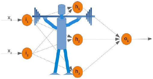
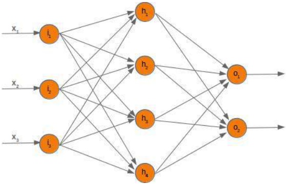
在接下来的章节中，我们将用 Python 设计一个包含三层的神经网络，即输入层、隐藏层和输出层。您可以在下面的图中看到这种神经网络结构。我们有一个包含三个节点 $i_1$,$i_2$,$i_3$ 的输入层。这些节点接收相应的输入值 $x_1$,$x_2$,$x_3$。中间或隐藏层有四个节点 $h_1$,$h_2$,$h_3$,$h_4$。这一层的输入源自输入层。我们很快就会讨论其机制。最后，我们的输出层由两个节点 $o_1$,$o_2$ 组成。

输入层与其他层不同。输入层的节点是被动的。这意味着输入神经元不会改变数据，即在这种情况下不使用权重。它们接收一个单一值并将其复制到多个输出中。

输入层由节点 $i_1$,$i_2$,$i_3$ 组成。原则上，输入是一个一维向量，例如 (2,4,11)。一维向量在 NumPy 中表示如下：

Python

import numpy as np input_vector = np.array([2, 4, 11]) print(input_vector)

输出：

[ 2 4 11]

在我们稍后编写的算法中，我们必须将其转置为列向量，即一个只有一列的二维数组：

Python

import numpy as np input_vector = np.array([2, 4, 11]) input_vector = np.array(input_vector, ndmin=2).T print("The input vector:\n", input_vector) print("The shape of this vector: ", input_vector.shape)

输出：

The input vector: [[ 2] [ 4] [11]] The shape of this vector: (3, 1)

权重与矩阵

我们网络图中的每条箭头都有一个相关的权重值。现在我们只看输入层和输出层之间的箭头。

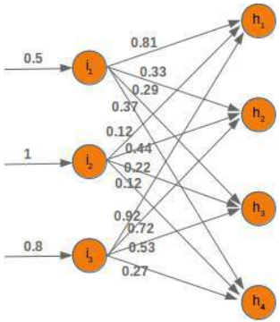
进入节点 $i_1$ 的值 $x_1$ 将根据权重值进行分配。在下面的图中，我们添加了一些示例值。使用这些值，隐藏层节点 ($h_1$,$h_2$,$h_3$,$h_4$) 的输入值 (I$h_1$,I$h_2$,I$h_3$,I$h_4$) 可以这样计算：

$Ih_1 = 0.81 * 0.5 + 0.12 * 1 + 0.92 * 0.8$

$Ih_2 = 0.33 * 0.5 + 0.44 * 1 + 0.72 * 0.8$

$Ih_3 = 0.29 * 0.5 + 0.22 * 1 + 0.53 * 0.8$

$Ih_4 = 0.37 * 0.5 + 0.12 * 1 + 0.27 * 0.8$

熟悉矩阵和矩阵乘法的人会明白这最终归结于什么。我们将重新绘制我们的网络并用 $w_ij$ 表示权重：

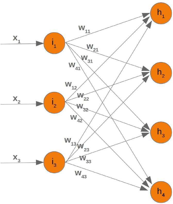
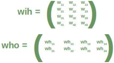
为了有效地执行所有必要的计算，我们将权重排列成一个权重矩阵。

我们上面图中的权重构成了一个数组，我们将在我们的神经网络类中将其命名为 'weights_in_hidden'。这个名称应该表明这些权重连接着输入节点和隐藏节点，也就是说，它们位于输入层和隐藏层之间。我们还会将其缩写为 'wih'。隐藏层和输出层之间的权重矩阵将表示为 "who"。

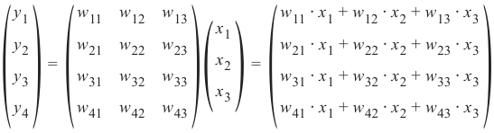
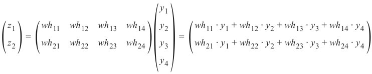
现在我们已经定义了权重矩阵，我们必须进行下一步。我们必须将矩阵 wih 乘以输入向量。顺便说一句，这正是我们在前面的示例中手动完成的。

对于隐藏层和输出层之间的 'who' 矩阵，我们也有类似的情况。因此，来自节点 $o_1$ 和 $o_2$ 的输出 $z_1$ 和 $z_2$ 也可以通过矩阵乘法计算：

您可能已经注意到我们之前的计算中缺少一些东西。我们在介绍性的“从零开始用 Python 构建神经网络”一章中展示过，我们必须对每个这些和应用一个激活函数或阶跃函数 Φ。

下图描绘了整个计算流程，即矩阵乘法和随后的激活函数应用。

矩阵 wih 和输入节点值 $x_1$,$x_2$,$x_3$ 矩阵之间的矩阵乘法计算出将传递给激活函数的输出。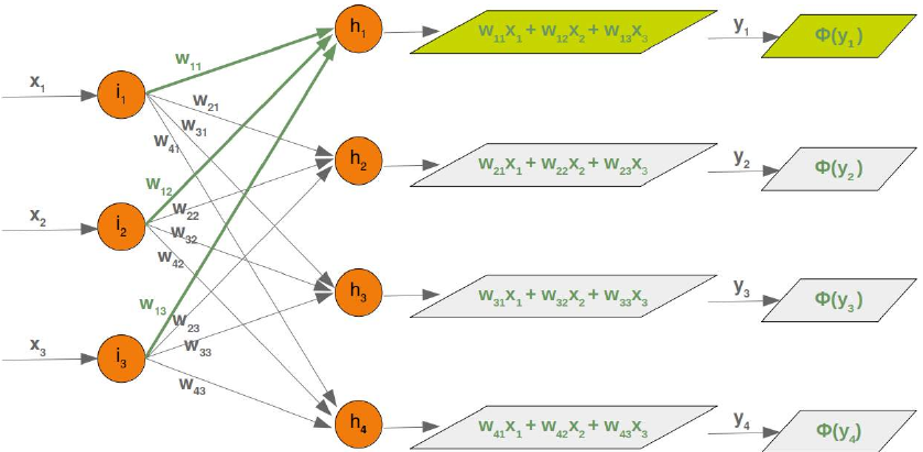

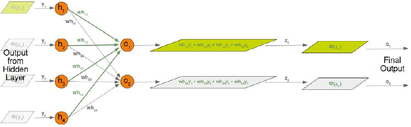
最终输出 $y_1$,$y_2$,$y_3$,$y_4$ 是权重矩阵 who 的输入：

尽管处理方式完全类似，但我们也将详细研究隐藏层和输出层之间发生的事情：

初始化权重矩阵

在训练神经网络之前，需要做出的重要选择之一是初始化权重矩阵。当我们开始时，我们对可能的权重一无所知。那么，我们可以从任意值开始吗？

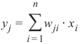
正如我们所看到的，除了输入节点之外，所有节点的输入都是通过对以下求和应用激活函数来计算的：

（其中 n 是前一层中的节点数，y_j 是到下一层节点的输入）

我们可以很容易地看到，将所有权重值设置为 0 并不是一个好主意，因为在这种情况下，这个求和的结果将始终为零。这意味着我们的网络将无法学习。这是最糟糕的选择，但将权重矩阵初始化为全 1 也是一个糟糕的选择。

权重矩阵的值应该随机选择，而不是任意选择。通过选择随机正态分布，我们打破了可能的对称情况，这对于学习过程来说可能并且通常是糟糕的。

有多种方法可以随机初始化权重矩阵。我们将介绍的第一种是来自 numpy.random 的均匀函数。它创建在半开区间 [low,high) 内均匀分布的样本，这意味着包含 low 但不包含 high。给定区间内的每个值被 'uniform' 抽取的可能性相同。

Python

import numpy as np number_of_samples = 1200 low = -1 high = 0 s = np.random.uniform(low, high, number_of_samples)

Python

# all values of s are within the half open interval [-1, 0) : print(np.all(s >= -1) and np.all(s < 0))

输出：True

在我们的上一个示例中，使用 uniform 函数创建的样本的直方图如下所示：

Python

import matplotlib.pyplot as plt plt.hist(s) plt.show()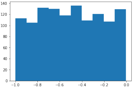

我们将看的下一个函数是 numpy.random 中的 binomial：

binomial(n, p, size=None)

它从具有指定参数的二项分布中抽取样本，n 次试验和成功概率 p，其中 n 是一个大于等于 0 的整数，p 是区间 [0,1] 中的浮点数。（n 可以输入为浮点数，但在使用时会被截断为整数）。

Python

s = np.random.binomial(100, 0.5, 1200) plt.hist(s) plt.show()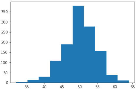

我们喜欢创建正态分布的随机数，但这些数字必须有界。np.random.normal() 不提供任何边界参数，因此不适用。

我们可以为此目的使用 scipy.stats 中的 truncnorm。

这种分布的标准形式是截断到范围 [a,b] 的标准正态分布——请注意，a 和 b 是在标准正态分布的域上定义的。要转换特定均值和标准差的剪切值，请使用：

$a, b = (m yc l i p_a - m y_m e an) / m y_s t d, (m yc l i p_b - m y_m e an) / m y_s t d$

Python

from scipy.stats import truncnorm s = truncnorm(a=-2/3., b=2/3., scale=1, loc=0).rvs(size=1000) plt.hist(s) plt.show()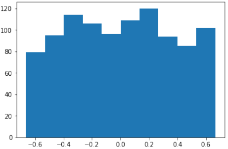

truncnorm 函数使用起来比较困难。为了简化操作，我们将在下面定义一个名为 truncated_normal 的函数，以便于完成此任务：

Python

def truncated_normal(mean=0, sd=1, low=0, upp=10): return truncnorm( (low - mean) / sd, (upp - mean) / sd, loc=mean, scale=sd) X = truncated_normal(mean=0, sd=0.4, low=-0.5, upp=0.5) s = X.rvs(10000) plt.hist(s) plt.show()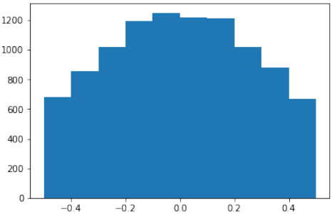

更多示例：

Python

X1 = truncated_normal(mean=2, sd=1, low=1, upp=10) X2 = truncated_normal(mean=5.5, sd=1, low=1, upp=10) X3 = truncated_normal(mean=8, sd=1, low=1, upp=10) import matplotlib.pyplot as plt fig, ax = plt.subplots(3, sharex=True) ax[0].hist(X1.rvs(10000), density=True) ax[1].hist(X2.rvs(10000), density=True) ax[2].hist(X3.rvs(10000), density=True) plt.show()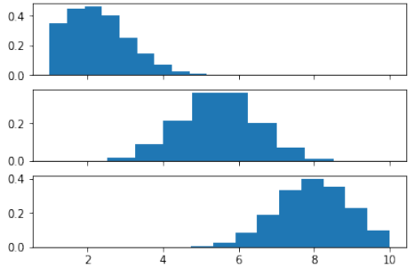

现在我们将创建链接权重矩阵。truncated_normal 非常适合此目的。最好从区间 $(−frac1s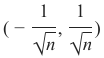qrtn,frac1sqrtn)$ 中选择随机值，其中 n 表示输入节点的数量。

因此，我们可以使用以下代码创建我们的 "wih" 矩阵：

Python

no_of_input_nodes = 3 no_of_hidden_nodes = 4 rad = 1 / np.sqrt(no_of_input_nodes) X = truncated_normal(mean=2, sd=1, low=-rad, upp=rad) wih = X.rvs((no_of_hidden_nodes, no_of_input_nodes)) wih

输出：

array([[-0.41379992, -0.24122842, -0.0303682 ], [ 0.07304837, -0.00160437, 0.0911987 ], [ 0.32405689, 0.5103896 , 0.23972997], [ 0.097932 , -0.06646741, 0.01359876]])

同样，我们现在可以定义 "who" 权重矩阵：

Python

no_of_hidden_nodes = 4 no_of_output_nodes = 2 rad = 1 / np.sqrt(no_of_hidden_nodes) # this is the input in this layer! X = truncated_normal(mean=2, sd=1, low=-rad, upp=rad) who = X.rvs((no_of_output_nodes, no_of_hidden_nodes)) who

输出：

array([[ 0.15892038, 0.06060043, 0.35900184, 0.14202827], [-0.4758216 , 0.29563269, 0.46035026, -0.29673539]])

INTRODUCTION
We introduced the basic ideas about
neural networks in the previous chapter of
our machine learning tutorial.
We have pointed out the similarity
between neurons and neural networks in
biology. We also introduced very small
articial neural networks and introduced
decision boundaries and the XOR
problem.
In the simple examples we introduced so
far, we saw that the weights are the
essential parts of a neural network. Before
we start to write a neural network with multiple layers, we need to have a closer look at the weights.
We have to see how to initialize the weights and how to efficiently multiply the weights with the input values.
In the following chapters we will design a neural network in Python, which consists of three layers, i.e. the
input layer, a hidden layer and an output layer. You can see this neural network structure in the following
diagram. We have an input layer with three nodes i 1, i 2, i 3 These nodes get the corresponding input values
x 1, x 2, x 3. The middle or hidden layer has four nodes h 1, h2, h 3, h 4. The input of this layer stems from the
input layer. We will discuss the mechanism soon. Finally, our output layer consists of the two nodes o 1, o2
The input layer is different from the other layers. The nodes of the input layer are passive. This means that the
input neurons do not change the data, i.e. there are no weights used in this case. They receive a single value
and duplicate this value to their many outputs.
141
The input layer consists of the nodes i 1, i 2 and i 3. In principle the input is a one-dimensional vector, like (2, 4,
11). A one-dimensional vector is represented in numpy like this:
import numpy as np
input_vector = np.array([2, 4, 11])
print(input_vector)
[ 2
4 11]
In the algorithm, which we will write later, we will have to transpose it into a column vector, i.e. a two-
dimensional array with just one column:
import numpy as np
input_vector = np.array([2, 4, 11])
input_vector = np.array(input_vector, ndmin=2).T
print("The input vector:\n", input_vector)
print("The shape of this vector: ", input_vector.shape)
The input vector:
[[ 2]
[ 4]
[11]]
The shape of this vector:
(3, 1)
142
WEIGHTS AND MATRICES
Each of the arrows in our network diagram has an associated weight value. We will only look at the arrows
between the input and the output layer now.
The value x1 going into the node i 1 will be distributed according to the values of the weights. In the following
diagram we have added some example values. Using these values, the input values (Ih 1, Ih 2, Ih 3, Ih 4 into the
nodes (h1, h 2, h 3, h 4) of the hidden layer can be calculated like this:
Ih 1 = 0.81 ∗ 0.5 + 0.12 ∗ 1 + 0.92 ∗ 0.8
Ih 2 = 0.33 ∗ 0.5 + 0.44 ∗ 1 + 0.72 ∗ 0.8
Ih 3 = 0.29 ∗ 0.5 + 0.22 ∗ 1 + 0.53 ∗ 0.8
Ih 4 = 0.37 ∗ 0.5 + 0.12 ∗ 1 + 0.27 ∗ 0.8
Those familiar with matrices and matrix multiplication will see where it is boiling down to. We will redraw
our network and denote the weights with wij:
143
In order to efficiently execute all the necessary calaculations, we will arrange the weights into a weight matrix.
144
The weights in our diagram above build an array, which we will call 'weights_in_hidden' in our Neural
Network class. The name should indicate that the weights are connecting the input and the hidden nodes, i.e.
they are between the input and the hidden layer. We will also abbreviate the name as 'wih'. The weight matrix
between the hidden and the output layer will be denoted as "who".:
Now that we have defined our weight matrices, we have to take the next step. We have to multiply the matrix
wih the input vector. Btw. this is exactly what we have manually done in our previous example.
( y y y y 4
1
2
3
) =
(
w w w w 31
41
11
21
w w w w 22
42
32
12
w w w w 13
33
23
43
) ( x3
x1
x2
) =
(
w w w w 41 31 21 11 ⋅ ⋅ ⋅ ⋅ x x x x 1 1 1 1 + + + + w w w w 12 42 22 32 ⋅ ⋅ ⋅ ⋅ x2 x x2 x2 2 + + + + w w13 w w 43 23 33 ⋅ ⋅ ⋅ ⋅ x x x x 3
3
3
3
)
We have a similar situation for the 'who' matrix between hidden and output layer. So the output z and z from
1 2the nodes o 1 and o 2 can also be calculated with matrix multiplications:
( z1
z2
) =
(
wh wh 11
21 wh wh 22
12
wh23 wh13 wh wh 14
24
) ( y y y y 4
1
2
3
)
=
(
wh21 wh 11 ⋅ ⋅ y1 y 1 + + wh wh 22 12 ⋅ ⋅ y y 2 2 + + wh wh 13 23 ⋅ ⋅ y3 y 3 + + wh wh 24 14 ⋅ ⋅ y y 4
4
)
You might have noticed that something is missing in our previous calculations. We showed in our introductory
145
chapter Neural Networks from Scratch in Python that we have to apply an activation or step function Φ on
each of these sums.
The following picture depicts the whole flow of calculation, i.e. the matrix multiplication and the succeeding
application of the activation function.
The matrix multiplication between the matrix wih and the matrix of the values of the input nodes x 1, x 2, x 3
calculates the output which will be passed to the activation function.
The final output y 1, y 2, y 3, y4 is the input of the weight matrix who:
Even though treatment is completely analogue, we will also have a detailled look at what is going on between
our hidden layer and the output layer:
146
INITIALIZING THE WEIGHT MATRICES
One of the important choices which have to be made before training a neural network consists in initializing
the weight matrices. We don't know anything about the possible weights, when we start. So, we could start
with arbitrary values?
As we have seen the input to all the nodes except the input nodes is calculated by applying the activation
function to the following sum:
n
y j = ∑ w ji ⋅ xi
i =1
(with n being the number of nodes in the previous layer and y j is the input to a node of the next layer)
We can easily see that it would not be a good idea to set all the weight values to 0, because in this case the
result of this summation will always be zero. This means that our network will be incapable of learning. This
is the worst choice, but initializing a weight matrix to ones is also a bad choice.
The values for the weight matrices should be chosen randomly and not arbitrarily. By choosing a random
normal distribution we have broken possible symmetric situations, which can and often are bad for the
learning process.
There are various ways to initialize the weight matrices randomly. The first one we will introduce is the unity
function from numpy.random. It creates samples which are uniformly distributed over the half-open interval
[low, high), which means that low is included and high is excluded. Each value within the given interval is
equally likely to be drawn by 'uniform'.
import numpy as np
number_of_samples = 1200
low = -1
high = 0
s = np.random.uniform(low, high, number_of_samples)
147
# all values of s are within the half open interval [-1, 0) :
print(np.all(s >= -1) and np.all(s < 0))
True
The histogram of the samples, created with the uniform function in our previous example, looks like this:
import matplotlib.pyplot as plt
plt.hist(s)
plt.show()
The next function we will look at is 'binomial' from numpy.binomial:
binomial(n, p, size=None)
It draws samples from a binomial distribution with specified parameters, n trials and probability p of
success where n is an integer >= 0 and p is a float in the interval [0,1]. ( n may be input as a float, but
it is truncated to an integer in use)
s = np.random.binomial(100, 0.5, 1200)
plt.hist(s)
plt.show()
148
We like to create random numbers with a normal distribution, but the numbers have to be bounded. This is not
the case with np.random.normal(), because it doesn't offer any bound parameter.
We can use truncnorm from scipy.stats for this purpose.
The standard form of this distribution is a standard normal truncated to the range [a, b] — notice that a and b
are defined over the domain of the standard normal. To convert clip values for a specific mean and standard
deviation, use:
a, b = (myclip_a - my_mean) / my_std, (myclip_b - my_mean) / my_std
from scipy.stats import truncnorm
s = truncnorm(a=-2/3., b=2/3., scale=1, loc=0).rvs(size=1000)
plt.hist(s)
plt.show()
149
The function 'truncnorm' is difficult to use. To make life easier, we define a function truncated_normal
in the following to fascilitate this task:
def truncated_normal(mean=0, sd=1, low=0, upp=10):
return truncnorm(
(low - mean) / sd, (upp - mean) / sd, loc=mean, scale=sd)
X = truncated_normal(mean=0, sd=0.4, low=-0.5, upp=0.5)
s = X.rvs(10000)
plt.hist(s)
plt.show()
Further examples:
150
X1 = truncated_normal(mean=2, sd=1, low=1, upp=10)
X2 = truncated_normal(mean=5.5, sd=1, low=1, upp=10)
X3 = truncated_normal(mean=8, sd=1, low=1, upp=10)
import matplotlib.pyplot as plt
fig, ax = plt.subplots(3, sharex=True)
ax[0].hist(X1.rvs(10000), density=True)
ax[1].hist(X2.rvs(10000), density=True)
ax[2].hist(X3.rvs(10000), density=True)
plt.show()
We will create the link weights matrix now. truncated_normal is ideal for this purpose. It is a good
idea to choose random values from within the interval
1
1
(−
,
)
√n √n
where n denotes the number of input nodes.
So we can create our "wih" matrix with:
no_of_input_nodes = 3
no_of_hidden_nodes = 4
rad = 1 / np.sqrt(no_of_input_nodes)
X = truncated_normal(mean=2, sd=1, low=-rad, upp=rad)
wih = X.rvs((no_of_hidden_nodes, no_of_input_nodes))
wih
151
Output:array([[-0.41379992, -0.24122842, -0.0303682 ],
[ 0.07304837, -0.00160437,
0.0911987 ],
[ 0.32405689, 0.5103896 ,
0.23972997],
[ 0.097932 , -0.06646741,
0.01359876]])
Similarly, we can now define the "who" weight matrix:
no_of_hidden_nodes = 4
no_of_output_nodes = 2
rad = 1 / np.sqrt(no_of_hidden_nodes)
# this is the input in thi
s layer!
X = truncated_normal(mean=2, sd=1, low=-rad, upp=rad)
who = X.rvs((no_of_output_nodes, no_of_hidden_nodes))
who
Output:array([[ 0.15892038,
0.06060043,
0.35900184, 0.14202827],
[-0.4758216 ,
0.29563269,
0.46035026, -0.29673539]])

Section outline

引言

权重与矩阵

初始化权重矩阵