神经网络中的反向传播(Backpropagation in Neural Networks)
章节大纲
-
引言
我们已经在之前的 Python 神经网络教程章节中介绍过。我们“运行神经网络”一章中的网络缺乏学习能力。它们只能在随机设置的权重值下运行。因此,我们无法用它们解决任何分类问题。然而,“简单神经网络”一章中的网络具有学习能力,但我们只将线性网络用于线性可分的类别。
当然,我们希望编写能够学习的通用 ANN(人工神经网络)。为此,我们必须理解反向传播 (backpropagation)。反向传播是一种常用的训练人工神经网络,特别是深度神经网络的方法。
反向传播是计算梯度 (gradient) 所必需的,我们需要梯度来调整权重矩阵的权重。我们网络中神经元(节点)的权重通过计算损失函数的梯度进行调整。为此,使用了梯度下降优化算法。它也称为误差反向传播。
人们常常被其中使用的数学吓退。我们试图用简单的术语来解释它。
许多文章或教程都以山来解释梯度下降。想象一下,你在夜晚或浓雾中被直升机放在一座山上,不一定是山顶。让我们进一步想象这座山在一个岛上,你想达到海平面。你必须下山,但你几乎什么也看不见,也许只有几米远。你的任务是找到下山的路,但你看不见小径。你可以使用梯度下降法。这意味着你正在检查你当前位置的陡峭程度。你将沿着最陡峭的下降方向前进。你只走几步,然后再次停下来重新定位。这意味着你再次应用前面描述的过程,即你正在寻找最陡峭的下降。
这个过程在下面的二维图中描绘。
这样继续下去,你将到达一个没有进一步下降的位置。
每个方向都向上。你可能已经达到了最深层——全局最小值,但你也可能被困在局部最小值中。如果你从我们图片右侧的位置开始,一切都很好,但从左侧开始,你将陷入局部最小值。
反向传播详解
现在,我们必须深入细节,即数学部分。
我们将从更简单的情况开始。我们来看一个线性网络。线性神经网络是指输出信号通过对所有加权输入信号求和而创建的网络。不会对这个和应用任何激活函数,这就是线性化的原因。
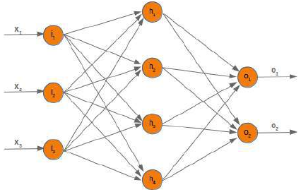
我们将使用以下简单的网络。
当我们训练网络时,我们有样本和相应的标签。对于每个输出值 \(o_i\),我们都有一个标签 \(t_i\),它是目标或期望值。如果标签等于输出,则结果正确,神经网络没有出错。原则上,误差是目标与实际输出之间的差异:
我们稍后将使用平方误差函数,因为它对算法具有更好的特性:
\[ e_i = \frac{(t_i - o_i)^2}{2} \]
我们想通过以下带有值的示例来阐明误差如何反向传播:
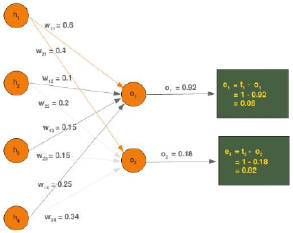
我们将看一下输出值 \(o_1\),它取决于值 \(w_11\),\(w_12\),\(w_13\)和 \(w_14\)。假设计算值 (\(o_1\)) 是 0.92,期望值 (\(t_1\)) 是 1。在这种情况下,误差是:
\[ e_1 = t_1 - o_1 = 1 - 0.92 = 0.08 \]
误差 \(e_2\) 可以这样计算:
\[ e_2 = t_2 - o_2 = 1 - 0.18 = 0.82 \]
根据这个误差,我们必须相应地改变传入值的权重。我们有四个权重,所以我们可以平均分配误差。然而,按比例分配更合理,即根据权重值进行分配。一个权重相对于其他权重越大,它对误差的责任就越大。这意味着我们可以将 \(w_{11}\) 中误差 \(e_1\) 的分数计算为:
\( e_1 \cdot \frac{w_{11}}{\sum_{i=1}^{4} w_{1i}} \)
这意味着在我们的示例中:
\(0.08 \cdot \frac{0.6}{ 0.6 + 0.1 + 0.15 + 0.25} = 0.0343 \)
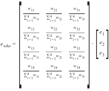
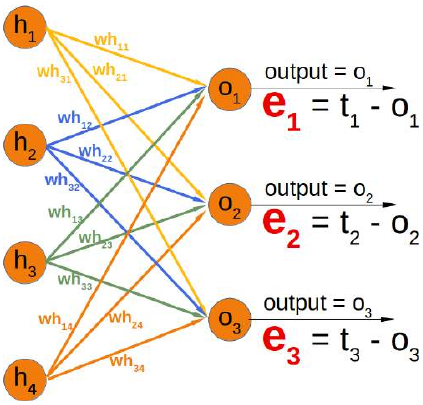
我们的隐藏层和输出层之间的权重矩阵——我们在上一章中称之为 'who' ——中的总误差如下所示:
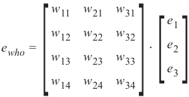
你可以看到左矩阵中的分母总是相同的。它起着缩放因子的作用。我们可以去掉它,这样计算会简单得多:
如果你将右侧的矩阵与我们“使用 Python 和 Numpy 的神经网络”一章中的 'who' 矩阵进行比较,你会发现它是 'who' 的转置。
\(e_{who}= {who.T} \cdot e\)
所以,这是线性神经网络的简单部分。我们到现在还没有考虑激活函数。
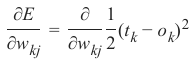
我们想在一个带有激活函数(即非线性网络)的网络中计算误差。误差函数的导数描述了斜率。正如我们在本章开头提到的,我们想要下降。导数描述了当权重 \(w_{kj}\)改变时,误差 E 如何变化:
\( \frac{\partial E}{\partial w_{kj}} \)
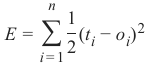
6666所有输出节点 \(o_i\)() 上的误差函数 E,其中 n 是输出节点的总数:
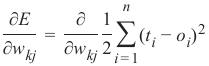
现在,我们可以将其插入到我们的导数中:
如果你看一下我们的示例网络,你会发现一个输出节点 \(o_k\)只取决于由权重 \(w_{ki}\)(其中 ,m 是隐藏节点的数量)创建的输入信号。
下图进一步阐明了这一点:
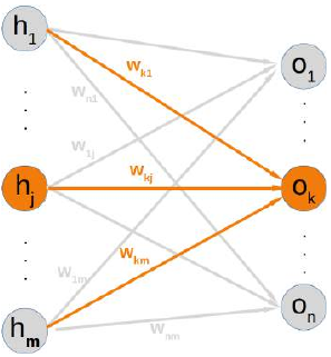
这意味着我们可以独立地计算每个输出节点的误差。这意味着我们可以从我们的求和中删除所有 (其中 )的表达式。因此,现在计算节点 k 的误差看起来简单得多:
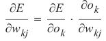
目标值 \(t_k\) 是一个常数,因为它不依赖于任何输入信号或权重。我们可以应用链式法则来对前面的项进行微分以简化事情:
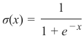
在我们教程的上一章中,我们使用 Sigmoid 函数作为激活函数:
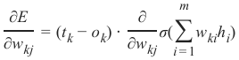
输出节点 \(o_k\)是通过对加权输入信号之和应用 Sigmoid 函数来计算的。这意味着我们可以通过用这个函数替换 \(o_k\)来进一步转换我们的导数项:
其中 m 是隐藏节点的数量。
Sigmoid 函数很容易求导:
现在完整的微分看起来像这样:
最后一部分必须对 \(w_{kj}\) 求导。这意味着所有乘积的导数都将为 0,除了项 \(w_{kj}\)\(h_j\),它对 \(w_{kj}\)的导数为 \(h_j\):
这就是我们需要在下一章中实现
NeuralNetwork类的train方法所需的一切。
INTRODUCTION
We already wrote in the previous chapters of our
tutorial on Neural Networks in Python. The networks
from our chapter Running Neural Networks lack the
capabilty of learning. They can only be run with
randomly set weight values. So we cannot solve any
classification problems with them. However, the
networks in Chapter Simple Neural Networks were
capable of learning, but we only used linear networks
for linearly separable classes.
Of course, we want to write general ANNs, which are
capable of learning. To do so, we will have to
understand backpropagation. Backpropagation is a
commonly used method for training artificial neural
networks, especially deep neural networks.
Backpropagation is needed to calculate the gradient,
which we need to adapt the weights of the weight matrices. The weight of the neuron (nodes) of our network
are adjusted by calculating the gradient of the loss function. For this purpose a gradient descent optimization
algorithm is used. It is also called backward propagation of errors.
Quite often people are frightened away by the mathematics used in it. We try to explain it in simple terms.
Explaining gradient descent starts in many articles or tutorials with mountains. Imagine you are put on a
mountain, not necessarily the top, by a helicopter at night or heavy fog. Let's further imagine that this
mountain is on an island and you want to reach sea level. You have to go down, but you hardly see anything,
maybe just a few metres. Your task is to find your way down, but you cannot see the path. You can use the
method of gradient descent. This means that you are examining the steepness at your current position. You
will proceed in the direction with the steepest descent. You take only a few steps and then you stop again to
reorientate yourself. This means you are applying again the previously described procedure, i.e. you are
looking for the steepest descend.
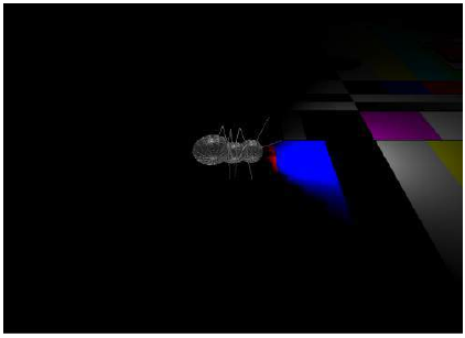
This procedure is depicted in the following diagram in a two-dimensional space.
162
Going on like this you will arrive at a position, where there is no further descend.
Each direction goes upwards. You may have reached the deepest level - the global minimum -, but you might
as well be stuck in a basin. If you start at the position on the right side of our image, everything works out fine,
but from the leftside, you will be stuck in a local minimum.
BACKPROPAGATION IN DETAIL
Now, we have to go into the details, i.e. the mathematics.
We will start with the simpler case. We look at a linear network. Linear neural networks are networks where
the output signal is created by summing up all the weighted input signals. No activation function will be
applied to this sum, which is the reason for the linearity.
The will use the following simple network.
When we are training the network we have samples and corresponding labels. For each output value o we
ihave a label t i, which is the target or the desired value. If the label is equal to the output, the result is correct
163
and the neural network has not made an error. Principially, the error is the difference between the target and
the actual output:
e i = t i − o i
We will later use a squared error function, because it has better characteristics for the algorithm:
1
e i =
(ti
− o i) 2
2We want to clarify how the error backpropagates with the following example with values:
We will have a look at the output value o 1, which is depending on the values w 11, w 12, w 13 and w 14. Let's
assume the calculated value (o 1) is 0.92 and the desired value (t 1) is 1. In this case the error is
e = t − o = 1 − 0.92 = 0.08
1 1 1The eror e 2 can be calculated like this:
e = t − o = 1 − 0.18 = 0.82
2 2 2164
Depending on this error, we have to change the weights from the incoming values accordingly. We have four
weights, so we could spread the error evenly. Yet, it makes more sense to to do it proportionally, according to
the weight values. The larger a weight is in relation to the other weights, the more it is responsible for the
error. This means that we can calculate the fraction of the error e 1 in w 11 as:
w11
e 1 ⋅
∑ 4 w 1i
i =1
This means in our example:
0.6
0.08 ⋅
= 0.0343
0.6 + 0.1 + 0.15 + 0.25
The total error in our weight matrix between the hidden and the output layer - we called it in our previous
chapter 'who' - looks like this
165
e who =
[ ∑ ∑ ∑ ∑ i 4 i 4 4 i i 4 w w w w =1
=1
=1
=1
13
12
11
14
w w w w 1i
1i
1i
1i
∑ ∑ ∑ ∑ i 4 i 4 i i 4 4 w24
w23
w21
w22
=1
=1
=1
=1
w w w w 2i
2i
2i
2i
∑ ∑ ∑ ∑ 4 4 i i i 4 i 4 w w w w =1
=1
=1
=1
31
32
34
33
w w w w 3i
3i
3i
3i
]
⋅
[ e3
e2
e1
]
You can see that the denominator in the left matrix is always the same. It functions like a scaling factor. We
can drop it so that the calculation gets a lot simpler:
e who =
[ w w w w 14
12
11
13
w w w w 22
23
24
21
w w w w 33
34
32
31
] ⋅
[ e e e 2
3
1
]
If you compare the matrix on the right side with the 'who' matrix of our chapter Neuronal Network Using
Python and Numpy, you will notice that it is the transpose of 'who'.
e who = who. T ⋅ e
So, this has been the easy part for linear neural networks. We haven't taken into account the activation function
until now.
We want to calculate the error in a network with an activation function, i.e. a non-linear network. The
derivation of the error function describes the slope. As we mentioned in the beginning of the this chapter, we
want to descend. The derivation describes how the error E changes as the weight w kj changes:
166
∂E
∂wkj
The error function E over all the output nodes o i (i = 1, . . . n) where n is the total number of output nodes:
n
1
E = ∑ (t i − o i) 2
2
i =1
Now, we can insert this in our derivation:
n
∂E
∂ 1
=
∑ (t i
− o i)2
∂wkj
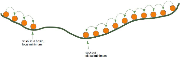
∂w kj 2 i = 1If you have a look at our example network, you will see that an output node o only depends on the input
ksignals created with the weights w ki with i = 1, ...m and m the number of hidden nodes.
The following diagram further illuminates this:
This means that we can calculate the error for every output node independently of each other. This means that
we can remove all expressions ti − oi with i ≠ k from our summation. So the calculation of the error for a node
k looks a lot simpler now:
∂E
∂ 1
=
(t k
− o k) 2
∂w ∂w 2kj
kjThe target value t k is a constant, because it is not depending on any input signals or weights. We can apply the
chain rule for the differentiation of the previous term to simplify things:
167
∂E
∂E
∂o k
=
⋅
∂w kj
∂o k
∂w kj
In the previous chapter of our tutorial, we used the sigmoid function as the activation function:
1
σ(x) =
1 + e − x
The output node o k is calculated by applying the sigmoid function to the sum of the weighted input signals.
This means that we can further transform our derivative term by replacing o by this function:
km
∂E
∂
= (tk − ok) ⋅
σ( ∑ w kih i
)
∂w kj
∂w kj i = 1where m is the number of hidden nodes.
The sigmoid function is easy to differentiate:
∂σ(x)
= σ(x) ⋅ (1 − σ(x))
∂x
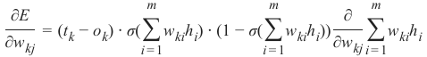
The complete differentiation looks like this now:
m
m
m
∂E
∂
= (t k − o k) ⋅ σ( ∑ w kih i) ⋅ (1 − σ( ∑ w kih i))
∑ w kih
i
∂w ∂wkj
i =1
i =1
kj i = 1The last part has to be differentiated with respect to w kj. This means that the derivation of all the products will
be 0 except the the term w kjh j) which has the derivative h j with respect to w kj:
m
m
∂E
= (tk − ok) ⋅ σ( ∑ w kih i) ⋅ (1 − σ( ∑ wkihi)) ⋅ h j
∂wkj
i =1
i =1
This is what we need to implement the method 'train' of our NeuralNetwork class in the following chapter.
In [ ]: