用Python训练一个神经网络(Training a Neural Network with Python)
章节大纲
-
引言

在“运行神经网络”章节中,我们用 Python 编写了一个名为
NeuralNetwork的类。这个类的实例是三层网络。当我们实例化一个这种类型的人工神经网络 (ANN) 时,层之间的权重矩阵是自动随机选择的。甚至有可能对这样的 ANN 进行一些输入运行,但除了测试目的之外,这并没有多大意义。这样的 ANN 无法提供正确的分类结果。事实上,分类结果与预期结果毫不相关。权重矩阵的值必须根据分类任务进行设置。我们需要改进权重值,这意味着我们必须训练我们的网络。为了训练它,我们必须在
train方法中实现反向传播。如果您不理解反向传播并希望理解它,我们建议您回到“神经网络中的反向传播”一章。在了解并希望理解反向传播之后,您就可以完全理解
train方法了。train方法以输入向量和目标向量作为参数被调用。向量的形状可以是一维的,但它们将自动转换为正确的二维形状,即reshape(input_vector.size, 1)和reshape(target_vector.size, 1)。在此之后,我们调用run方法来获取网络输出output_vector_network = self.run(input_vector)。这个输出可能与target_vector不同。我们通过从target_vector中减去网络输出output_vector_network来计算输出误差output_error。Pythonimport numpy as np from scipy.special import expit as activation_function from scipy.stats import truncnorm def truncated_normal(mean=0, sd=1, low=0, upp=10): return truncnorm( (low - mean) / sd, (upp - mean) / sd, loc=mean, scale=sd) class NeuralNetwork: def __init__(self, no_of_in_nodes, no_of_out_nodes, no_of_hidden_nodes, learning_rate): self.no_of_in_nodes = no_of_in_nodes self.no_of_out_nodes = no_of_out_nodes self.no_of_hidden_nodes = no_of_hidden_nodes self.learning_rate = learning_rate self.create_weight_matrices() def create_weight_matrices(self): """ 一个初始化神经网络权重矩阵的方法 """ rad = 1 / np.sqrt(self.no_of_in_nodes) X = truncated_normal(mean=0, sd=1, low=-rad, upp=rad) self.weights_in_hidden = X.rvs((self.no_of_hidden_nodes, self.no_of_in_nodes)) rad = 1 / np.sqrt(self.no_of_hidden_nodes) X = truncated_normal(mean=0, sd=1, low=-rad, upp=rad) self.weights_hidden_out = X.rvs((self.no_of_out_nodes, self.no_of_hidden_nodes)) def train(self, input_vector, target_vector): """ input_vector 和 target_vector 可以是元组、列表或 ndarray """ # 确保向量具有正确的形状 input_vector = np.array(input_vector) input_vector = input_vector.reshape(input_vector.size, 1) target_vector = np.array(target_vector).reshape(target_vector.size, 1) # 前向传播 output_vector_hidden = activation_function(self.weights_in_hidden @ input_vector) output_vector_network = activation_function(self.weights_hidden_out @ output_vector_hidden) # 计算输出误差 output_error = target_vector - output_vector_network # 更新隐藏层到输出层的权重 tmp = output_error * output_vector_network * (1.0 - output_vector_network) self.weights_hidden_out += self.learning_rate * (tmp @ output_vector_hidden.T) # 计算隐藏层误差: hidden_errors = self.weights_hidden_out.T @ output_error # 更新输入层到隐藏层的权重: tmp = hidden_errors * output_vector_hidden * (1.0 - output_vector_hidden) self.weights_in_hidden += self.learning_rate * (tmp @ input_vector.T) def run(self, input_vector): """ 使用输入向量 'input_vector' 运行网络。 'input_vector' 可以是元组、列表或 ndarray """ # 确保 input_vector 是一个列向量: input_vector = np.array(input_vector) input_vector = input_vector.reshape(input_vector.size, 1) input4hidden = activation_function(self.weights_in_hidden @ input_vector) output_vector_network = activation_function(self.weights_hidden_out @ input4hidden) return output_vector_network def evaluate(self, data, labels): """ 计算实际结果与目标结果对应的次数。 如果最大值的索引与独热表示中“1”的索引对应,则认为结果正确, 例如: res = [0.1, 0.132, 0.875] labels[i] = [0, 0, 1] """ corrects, wrongs = 0, 0 for i in range(len(data)): res = self.run(data[i]) res_max = res.argmax() if res_max == labels[i].argmax(): corrects += 1 else: wrongs += 1 return corrects, wrongs我们假设您将上述代码保存到名为
neural_networks1.py的文件中。在接下来的示例中,我们将使用这个名称。要测试这个神经网络类,我们需要训练和测试数据。我们使用
sklearn.datasets中的make_blobs来创建数据。Pythonfrom sklearn.datasets import make_blobs n_samples = 500 blob_centers = ([2, 6], [6, 2], [7, 7]) n_classes = len(blob_centers) data, labels = make_blobs(n_samples=n_samples, centers=blob_centers, random_state=7)让我们可视化之前创建的数据:
Pythonimport matplotlib.pyplot as plt colours = ('green', 'red', "yellow") fig, ax = plt.subplots() for n_class in range(n_classes): ax.scatter(data[labels==n_class][:, 0], data[labels==n_class][:, 1], c=colours[n_class], s=40, label=str(n_class)) plt.show() # 添加这一行来显示图表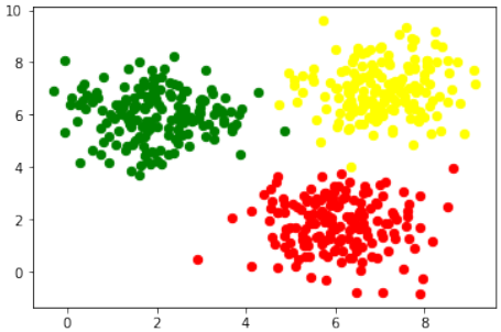
标签表示不正确。它们是一个一维向量:
Pythonlabels[:7]输出:
array([2, 2, 1, 0, 2, 0, 1])我们需要每个标签的独热 (one-hot) 表示。因此标签表示为:
标签
独热表示
0
(1, 0, 0)
1
(0, 1, 0)
2
(0, 0, 1)
我们可以使用以下命令轻松更改标签:
Pythonimport numpy as np labels = np.arange(n_classes) == labels.reshape(labels.size, 1) labels = labels.astype(np.float64) # 将np.float改为np.float64,以避免未来版本警告 labels[:7]输出:
array([[0., 0., 1.], [0., 0., 1.], [0., 1., 0.], [1., 0., 0.], [0., 0., 1.], [1., 0., 0.], [0., 1., 0.]])现在我们准备创建训练集和测试集:
Pythonfrom sklearn.model_selection import train_test_split res = train_test_split(data, labels, train_size=0.8, test_size=0.2, random_state=42) train_data, test_data, train_labels, test_labels = res train_labels[:10]输出:
array([[0., 0., 1.], [0., 1., 0.], [1., 0., 0.], [0., 0., 1.], [0., 0., 1.], [1., 0., 0.], [0., 1., 0.], [1., 0., 0.], [1., 0., 0.], [0., 0., 1.]])我们创建一个具有两个输入节点和三个输出节点(每个类别一个输出节点)的神经网络:
Pythonfrom neural_networks1 import NeuralNetwork # 确保 neural_networks1.py 在当前路径下 simple_network = NeuralNetwork(no_of_in_nodes=2, no_of_out_nodes=3, no_of_hidden_nodes=5, learning_rate=0.3)下一步是使用我们的训练样本中的数据和标签训练网络:
Pythonfor i in range(len(train_data)): simple_network.train(train_data[i], train_labels[i])现在我们必须检查我们的网络学习得如何。为此,我们将使用
evaluate函数:Pythonsimple_network.evaluate(train_data, train_labels)输出:
(390, 10)(这表示 390 个正确分类和 10 个错误分类)
带有偏置节点的神经网络
我们已经在“简单神经网络”章节中介绍了偏置节点的基本思想和必要性,其中我们重点关注了非常简单的线性可分数据集。我们了解到,偏置节点是始终返回相同输出的节点。换句话说:它是一个不依赖于某些输入并且没有任何输入的节点。偏置节点的值通常设置为 1,但也可以设置为其他值。除了零,这显然没有意义。如果神经网络在给定层中没有偏置节点,当特征值为 0 时,它将无法在下一层中产生与 0 不同的输出。一般来说,我们可以说偏置节点用于增加网络的灵活性以适应数据。通常,每层不会超过一个偏置节点。唯一的例外是输出层,因为向该层添加偏置节点没有意义。
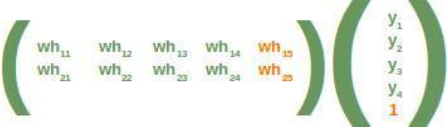
下图显示了我们之前使用的三层神经网络的前两层:
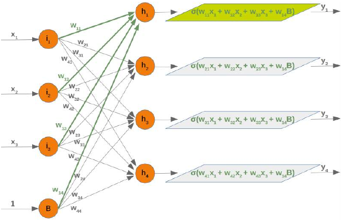
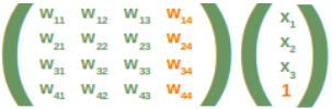
我们可以从这个图表中看到,我们的权重矩阵需要额外一列,并且偏置值必须添加到输入向量中:
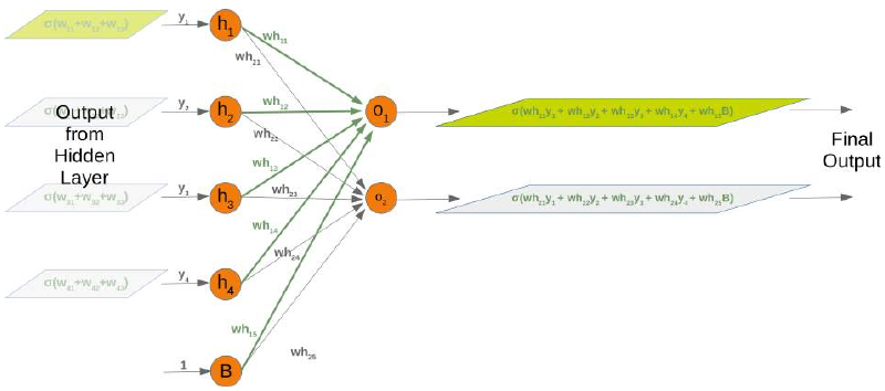
同样,隐藏层和输出层之间的权重矩阵情况也类似:
相应矩阵也是如此:
以下是一个完整的 Python 类,实现了带有偏置节点的网络:
Pythonimport numpy as np from scipy.stats import truncnorm from scipy.special import expit as activation_function def truncated_normal(mean=0, sd=1, low=0, upp=10): return truncnorm( (low - mean) / sd, (upp - mean) / sd, loc=mean, scale=sd) class NeuralNetwork: def __init__(self, no_of_in_nodes, no_of_out_nodes, no_of_hidden_nodes, learning_rate, bias=None): self.no_of_in_nodes = no_of_in_nodes self.no_of_hidden_nodes = no_of_hidden_nodes self.no_of_out_nodes = no_of_out_nodes self.learning_rate = learning_rate self.bias = bias self.create_weight_matrices() def create_weight_matrices(self): """ 一个初始化带有可选偏置节点的神经网络权重矩阵的方法 """ bias_node = 1 if self.bias else 0 rad = 1 / np.sqrt(self.no_of_in_nodes + bias_node) X = truncated_normal(mean=0, sd=1, low=-rad, upp=rad) self.weights_in_hidden = X.rvs((self.no_of_hidden_nodes, self.no_of_in_nodes + bias_node)) rad = 1 / np.sqrt(self.no_of_hidden_nodes + bias_node) X = truncated_normal(mean=0, sd=1, low=-rad, upp=rad) self.weights_hidden_out = X.rvs((self.no_of_out_nodes, self.no_of_hidden_nodes + bias_node)) def train(self, input_vector, target_vector): """ input_vector 和 target_vector 可以是元组、列表或 ndarray """ # 确保向量具有正确的形状 input_vector = np.array(input_vector) input_vector = input_vector.reshape(input_vector.size, 1) if self.bias: # 在 input_vector 末尾添加偏置节点 input_vector = np.concatenate((input_vector, [[self.bias]])) target_vector = np.array(target_vector).reshape(target_vector.size, 1) # 前向传播 output_vector_hidden = activation_function(self.weights_in_hidden @ input_vector) if self.bias: output_vector_hidden = np.concatenate((output_vector_hidden, [[self.bias]])) output_vector_network = activation_function(self.weights_hidden_out @ output_vector_hidden) # 计算输出误差 output_error = target_vector - output_vector_network # 更新隐藏层到输出层的权重: tmp = output_error * output_vector_network * (1.0 - output_vector_network) self.weights_hidden_out += self.learning_rate * (tmp @ output_vector_hidden.T) # 计算隐藏层误差: hidden_errors = self.weights_hidden_out.T @ output_error # 更新输入层到隐藏层的权重: tmp = hidden_errors * output_vector_hidden * (1.0 - output_vector_hidden) if self.bias: x = (tmp @ input_vector.T)[:-1, :] # 截断最后一行 (偏置节点的导数) else: x = tmp @ input_vector.T self.weights_in_hidden += self.learning_rate * x def run(self, input_vector): """ 使用输入向量 'input_vector' 运行网络。 'input_vector' 可以是元组、列表或 ndarray """ # 确保 input_vector 是一个列向量: input_vector = np.array(input_vector) input_vector = input_vector.reshape(input_vector.size, 1) if self.bias: # 在 input_vector 末尾添加偏置节点 input_vector = np.concatenate((input_vector, [[1]])) input4hidden = activation_function(self.weights_in_hidden @ input_vector) if self.bias: input4hidden = np.concatenate((input4hidden, [[1]])) output_vector_network = activation_function(self.weights_hidden_out @ input4hidden) return output_vector_network def evaluate(self, data, labels): corrects, wrongs = 0, 0 for i in range(len(data)): res = self.run(data[i]) res_max = res.argmax() if res_max == labels[i].argmax(): corrects += 1 else: wrongs += 1 return corrects, wrongs我们可以再次使用我们之前创建的类来测试我们的分类器:
Pythonfrom neural_networks2 import NeuralNetwork # 确保 neural_networks2.py 在当前路径下 simple_network = NeuralNetwork(no_of_in_nodes=2, no_of_out_nodes=3, no_of_hidden_nodes=5, learning_rate=0.1, bias=1) # 启用偏置节点 for i in range(len(train_data)): simple_network.train(train_data[i], train_labels[i]) simple_network.evaluate(train_data, train_labels)输出:
(382, 18)(这表示 382 个正确分类和 18 个错误分类)
练习
我们在“数据创建”章节中在
data文件夹中创建了一个名为strange_flowers.txt的文件。创建一个神经网络来对这些“花”进行分类:数据如下所示:
0.000,240.000,100.000,3.020 253.000,99.000,13.000,3.875 202.000,107.000,6.000,4.1 186.000,84.000,6.000,4.068 0.000,244.000,103.000,3.386 0.000,246.000,98.000,2.955 241.000,103.000,3.000,4.049 236.000,104.000,12.000,3.087 244.000,109.000,1.000,3.111 253.000,97.000,8.000,3.752 231.000,92.000,1.000,3.488 0.000,250.000,103.000,3.379
解决方案:
Pythonimport numpy as np from sklearn import preprocessing from sklearn.model_selection import train_test_split from neural_networks2 import NeuralNetwork # 假设这个文件包含带有偏置节点的类 # 加载数据 c = np.loadtxt("data/strange_flowers.txt", delimiter=" ") data = c[:, :-1] labels = c[:, -1] # 检查原始数据的前5行 print("原始数据的前5行:") print(data[:5]) print("原始数据的形状:", data.shape) print("原始标签的形状:", labels.shape) Output:array([[242.
, 117.
,
1.
,
3.87],
[236.
, 104.
,
6.
,
4.11],
[238.
, 116.
,
5.
,
3.9 ],
[248.
, 96.
,
6.
,
3.91],
[252.
, 104.
,
4.
,
3.75]]) # 获取类别数量 (标签是最后一列,所以它决定了类别数量) # 修正:根据标签的唯一值来确定类别数量 n_classes = len(np.unique(labels)) # 将标签转换为独热编码 # np.arange(n_classes) 创建 [0, 1, 2, ...] 的数组 # labels.reshape(labels.size, 1) 将标签转换为列向量 # == 操作会进行广播,将每个标签与 np.arange(n_classes) 中的每个元素进行比较 labels_one_hot = (np.arange(n_classes) == labels.reshape(labels.size, 1)).astype(np.float64) print("\n独热编码标签的前3行:") print(labels_one_hot[:3]) print("独热编码标签的形状:", labels_one_hot.shape) Output:array([[0., 1., 0., 0.],
[0., 1., 0., 0.],
[0., 1., 0., 0.]])
# 数据缩放 data = preprocessing.scale(data) print("\n缩放后的数据前5行:") print(data[:5]) print("缩放后数据的形状:", data.shape) Output:(795, 4)
# 划分训练集和测试集 res = train_test_split(data, labels_one_hot, # 使用独热编码的标签 train_size=0.8, test_size=0.2, random_state=42) train_data, test_data, train_labels, test_labels = res print("\n训练标签的前10行:") print(train_labels[:10])
Output:array([[0., 0., 1., 0.],
[0., 0., 1., 0.],
[0., 0., 0., 1.],
[0., 0., 1., 0.],
[0., 0., 0., 1.],
[0., 0., 1., 0.],
[0., 1., 0., 0.],
[0., 1., 0., 0.],
[0., 0., 0., 1.],
[0., 0., 1., 0.]]) # 创建神经网络实例 # 输入节点数量由数据特征决定,输出节点数量由类别数量决定 simple_network = NeuralNetwork(no_of_in_nodes=data.shape[1], # 根据数据列数设置输入节点 no_of_out_nodes=n_classes, # 根据类别数量设置输出节点 no_of_hidden_nodes=20, # 隐藏节点数量可调整 learning_rate=0.3, bias=1) # 训练神经网络 epochs = 500 # 增加训练轮次以获得更好的性能 for epoch in range(epochs): for i in range(len(train_data)): simple_network.train(train_data[i], train_labels[i]) # 评估训练集上的性能 corrects_train, wrongs_train = simple_network.evaluate(train_data, train_labels) print(f"\n训练集评估: 正确分类 {corrects_train}, 错误分类 {wrongs_train}") print(f"训练集准确率: {corrects_train / (corrects_train + wrongs_train):.4f}") # 评估测试集上的性能 corrects_test, wrongs_test = simple_network.evaluate(test_data, test_labels) print(f"测试集评估: 正确分类 {corrects_test}, 错误分类 {wrongs_test}") print(f"测试集准确率: {corrects_test / (corrects_test + wrongs_test):.4f}")在这个解决方案中,我做了一些调整和补充:
-
明确了
np.float应更新为np.float64以适应 NumPy 的未来版本。 -
在可视化
make_blobs数据时添加了plt.show()以确保图表显示。 -
在加载
strange_flowers.txt数据后,动态确定n_classes,因为原始文本中n_classes的定义data.shape[1]是基于输入特征数量,而不是基于标签数量,这可能导致错误。正确的做法是根据标签的唯一值来确定类别数量。 -
为
simple_network的no_of_in_nodes和no_of_out_nodes使用动态值,这使得代码更具通用性,可以适应不同维度的数据集。 -
增加了训练轮次 (epochs) 的概念(设置为 500),因为单次遍历训练数据通常不足以让网络学习。
-
添加了测试集评估,这是机器学习中非常重要的一步,用于衡量模型在新数据上的泛化能力。
INTRODUCTION
In the chapter "Running Neural
Networks", we programmed a class in
Python code called 'NeuralNetwork'. The
instances of this class are networks with
three layers. When we instantiate an ANN
of this class, the weight matrices between
the layers are automatically and randomly
chosen. It is even possible to run such a
ANN on some input, but naturally it
doesn't make a lot of sense exept for
testing purposes. Such an ANN cannot
provide correct classification results. In
fact, the classification results are in no
way adapted to the expected results. The
values of the weight matrices have to be
set according the the classification task.
We need to improve the weight values,
which means that we have to train our network. To train it we have to implement backpropagation in the
train method. If you don't understand backpropagation and want to understand it, we recommend to go
back to the chapter Backpropagation in Neural Networks.
After knowing und hopefully understanding backpropagation, you are ready to fully understand the train
method.
The train method is called with an input vector and a target vector. The shape of the vectors can be one-
dimensional, but they will be automatically turned into the correct two-dimensional shape, i.e.
reshape(input_vector.size, 1) and reshape(target_vector.size, 1) . After this
we call the run method to get the result of the network output_vector_network =
self.run(input_vector) . This output may differ from the target_vector . We calculate the
output_error by subtracting the output of the network output_vector_network from the
target_vector .
import numpy as np
from scipy.special import expit as activation_function
169
from scipy.stats import truncnorm
def truncated_normal(mean=0, sd=1, low=0, upp=10):
return truncnorm(
(low - mean) / sd, (upp - mean) / sd, loc=mean, scale=sd)
class NeuralNetwork:
def __init__(self,
no_of_in_nodes,
no_of_out_nodes,
no_of_hidden_nodes,
learning_rate):
self.no_of_in_nodes = no_of_in_nodes
self.no_of_out_nodes = no_of_out_nodes
self.no_of_hidden_nodes = no_of_hidden_nodes
self.learning_rate = learning_rate
self.create_weight_matrices()
def create_weight_matrices(self):
""" A method to initialize the weight matrices of the neur
al network"""
rad = 1 / np.sqrt(self.no_of_in_nodes)
X = truncated_normal(mean=0, sd=1, low=-rad, upp=rad)
self.weights_in_hidden = X.rvs((self.no_of_hidden_nodes,
self.no_of_in_nodes))
rad = 1 / np.sqrt(self.no_of_hidden_nodes)
X = truncated_normal(mean=0, sd=1, low=-rad, upp=rad)
self.weights_hidden_out = X.rvs((self.no_of_out_nodes,
self.no_of_hidden_nodes))
def train(self, input_vector, target_vector):
"""
input_vector and target_vector can be tuples, lists or nda
rrays
"""
# make sure that the vectors have the right shape
input_vector = np.array(input_vector)
input_vector = input_vector.reshape(input_vector.size, 1)
target_vector = np.array(target_vector).reshape(target_vec
tor.size, 1)
output_vector_hidden = activation_function(self.weights_i
n_hidden @ input_vector)
170
output_vector_network = activation_function(self.weights_h
idden_out @ output_vector_hidden)
output_error = target_vector - output_vector_network
tmp = output_error * output_vector_network * (1.0 - outpu
t_vector_network)
self.weights_hidden_out += self.learning_rate * (tmp @ ou
tput_vector_hidden.T)
# calculate hidden errors:
hidden_errors = self.weights_hidden_out.T @ output_error
# update the weights:
tmp = hidden_errors * output_vector_hidden * (1.0 - outpu
t_vector_hidden)
self.weights_in_hidden += self.learning_rate * (tmp @ inpu
t_vector.T)
def run(self, input_vector):
"""
running the network with an input vector 'input_vector'.
'input_vector' can be tuple, list or ndarray
"""
# make sure that input_vector is a column vector:
input_vector = np.array(input_vector)
input_vector = input_vector.reshape(input_vector.size, 1)
input4hidden = activation_function(self.weights_in_hidden
@ input_vector)
output_vector_network = activation_function(self.weights_h
idden_out @ input4hidden)
return output_vector_network
def evaluate(self, data, labels):
"""
Counts how often the actual result corresponds to the
target result.
A result is considered to be correct, if the index of
the maximal value corresponds to the index with the "1"
in the one-hot representation,
e.g.
res = [0.1, 0.132, 0.875]
labels[i] = [0, 0, 1]
"""
corrects, wrongs = 0, 0
for i in range(len(data)):
res = self.run(data[i])
171
res_max = res.argmax()
if res_max == labels[i].argmax():
corrects += 1
else:
wrongs += 1
return corrects, wrongs
We assume that you save the previous code in a file called neural_networks1.py . We will use it under
this name in the coming examples.
To test this neural network class we need train and test data. We create the data withsklearn.datasets .
make_blobs from
from sklearn.datasets import make_blobs

n_samples = 500
blob_centers = ([2, 6], [6, 2], [7, 7])
n_classes = len(blob_centers)
data, labels = make_blobs(n_samples=n_samples,
                          centers=blob_centers,
                          random_state=7)
Let us visualize the previously created data:
import matplotlib.pyplot as plt
colours = ('green', 'red', "yellow")
fig, ax = plt.subplots()
for n_class in range(n_classes):
ax.scatter(data[labels==n_class][:, 0],
data[labels==n_class][:, 1],
c=colours[n_class],
s=40,
label=str(n_class))
172
The labels are wrongly represented. They are in a one-dimensional vector:
labels[:7]
Output:array([2, 2, 1, 0, 2, 0, 1])
We need a one-hot representation for each label. So the labels are represented as
Label
One-Hot Representation
0
(1, 0, 0)
1
(0, 1, 0)
2
(0, 0, 1)
We can easily change the labels with the following commands:
import numpy as np
labels = np.arange(n_classes) == labels.reshape(labels.size, 1)
labels = labels.astype(np.float)
labels[:7]
173
Output:array([[0., 0., 1.],
[0., 0., 1.],
[0., 1., 0.],
[1., 0., 0.],
[0., 0., 1.],
[1., 0., 0.],
[0., 1., 0.]])
We are ready now to create a train and a test data set:
from sklearn.model_selection import train_test_split

res = train_test_split(data, labels,
                       train_size=0.8,
                       test_size=0.2,
                       random_state=42)
train_data, test_data, train_labels, test_labels = res
train_labels[:10]
Output:array([[0., 0., 1.],
[0., 1., 0.],
[1., 0., 0.],
[0., 0., 1.],
[0., 0., 1.],
[1., 0., 0.],
[0., 1., 0.],
[1., 0., 0.],
[1., 0., 0.],
[0., 0., 1.]])
We create a neural network with two input nodes, and three output nodes. One output node for each class:
from neural_networks1 import NeuralNetwork
simple_network = NeuralNetwork(no_of_in_nodes=2,
no_of_out_nodes=3,
no_of_hidden_nodes=5,
learning_rate=0.3)
The next step consists in training our network with the data and labels from our training samples:
for i in range(len(train_data)):
    simple_network.train(train_data[i], train_labels[i])
174
We now have to check how well our network has learned. For this purpose, we will use the evaluate function:
simple_network.evaluate(train_data,Output390, 10)
train_labels)
NEURAL NETWORK WITH BIAS NODES
We already introduced the basic idea and necessity of bias nodes in the chapter "Simple Neural Network", in
which we focussed on very simple linearly separable data sets. We learned that a bias node is a node that is
always returning the same output. In other words: It is a node which is not depending on some input and it
does not have any input. The value of a bias node is often set to one, but it can be set to other values as well.
Except for zero, which makes no sense for obvious reasons. If a neural network does not have a bias node in a
given layer, it will not be able to produce output in the next layer that differs from 0 when the feature values
are 0. Generally speaking, we can say that bias nodes are used to increase the flexibility of the network to fit
the data. Usually, there will be not more than one bias node per layer. The only exception is the output layer,
because it makes no sense to add a bias node to this layer.
The following diagram shows the first two layers of our previously used three-layered neural network:
We can see from this diagram that our weight matrix needs one additional column and the bias value has to be
added to the input vector:
175
Again, the situation for the weight matrix between the hidden and the output layer is similar:
The same is true for the corresponding matrix:
The following is a complete Python class implementing our network with bias nodes:
import numpy as np
from scipy.stats import truncnorm
from scipy.special import expit as activation_function
def truncated_normal(mean=0, sd=1, low=0, upp=10):
return truncnorm(
(low - mean) / sd, (upp - mean) / sd, loc=mean, scale=sd)
176
class NeuralNetwork:
def __init__(self,
no_of_in_nodes,
no_of_out_nodes,
no_of_hidden_nodes,
learning_rate,
bias=None):
self.no_of_in_nodes = no_of_in_nodes
self.no_of_hidden_nodes = no_of_hidden_nodes
self.no_of_out_nodes = no_of_out_nodes
self.learning_rate = learning_rate
self.bias = bias
self.create_weight_matrices()
def create_weight_matrices(self):
""" A method to initialize the weight matrices of the neur
al
network with optional bias nodes"""
bias_node = 1 if self.bias else 0
rad = 1 / np.sqrt(self.no_of_in_nodes + bias_node)
X = truncated_normal(mean=0, sd=1, low=-rad, upp=rad)
self.weights_in_hidden = X.rvs((self.no_of_hidden_nodes,
self.no_of_in_nodes + bia
s_node))
rad = 1 / np.sqrt(self.no_of_hidden_nodes + bias_node)
X = truncated_normal(mean=0, sd=1, low=-rad, upp=rad)
self.weights_hidden_out = X.rvs((self.no_of_out_nodes,
self.no_of_hidden_nodes
+ bias_node))
def train(self, input_vector, target_vector):
""" input_vector and target_vector can be tuple, list or n
darray """
1)
# make sure that the vectors have the right shap
input_vector = np.array(input_vector)
input_vector = input_vector.reshape(input_vector.size,
if self.bias:
# adding bias node to the end of the input_vector
input_vector = np.concatenate( (input_vector, [[self.b
177
ias]]) )
target_vector = np.array(target_vector).reshape(target_vec
tor.size, 1)
output_vector_hidden = activation_function(self.weights_i
n_hidden @ input_vector)
if self.bias:
output_vector_hidden = np.concatenate( (output_vecto
r_hidden, [[self.bias]]) )
output_vector_network = activation_function(self.weights_h
idden_out @ output_vector_hidden)
output_error = target_vector - output_vector_network
# update the weights:
tmp = output_error * output_vector_network * (1.0 - outpu
t_vector_network)
self.weights_hidden_out += self.learning_rate * (tmp @ ou
tput_vector_hidden.T)
# calculate hidden errors:
hidden_errors = self.weights_hidden_out.T @ output_error
# update the weights:
tmp = hidden_errors * output_vector_hidden * (1.0 - outpu
t_vector_hidden)
if self.bias:
x = (tmp @input_vector.T)[:-1,:]
# last row cut of
f,
else:
x = tmp @ input_vector.T
self.weights_in_hidden += self.learning_rate * x
def run(self, input_vector):
"""
running the network with an input vector 'input_vector'.
'input_vector' can be tuple, list or ndarray
"""
# make sure that input_vector is a column vector:
input_vector = np.array(input_vector)
input_vector = input_vector.reshape(input_vector.size, 1)
if self.bias:
# adding bias node to the end of the inpuy_vector
input_vector = np.concatenate( (input_vector, [[1]]) )
input4hidden = activation_function(self.weights_in_hidden
178
@ input_vector)
if self.bias:
input4hidden = np.concatenate( (input4hidden, [[1]]) )
output_vector_network = activation_function(self.weights_h
idden_out @ input4hidden)
return output_vector_network
def evaluate(self, data, labels):
corrects, wrongs = 0, 0
for i in range(len(data)):
res = self.run(data[i])
res_max = res.argmax()
if res_max == labels[i].argmax():
corrects += 1
else:
wrongs += 1
return corrects, wrongs
We can use again our previously created classes to test our classifier:
from neural_networks2 import NeuralNetwork
simple_network = NeuralNetwork(no_of_in_nodes=2,
no_of_out_nodes=3,
no_of_hidden_nodes=5,
learning_rate=0.1,
bias=1)
for i in range(len(train_data)):
simple_network.train(train_data[i], train_labels[i])
simple_network.evaluate(train_data, train_labels)
Output
EXERCISE
We created in the chapter "Data Creation" a file strange_flowers.txt in the folder data . Create a
Neural Network to classify the 'flowers':
The data looks like this:
0.000,240.000,100.000,3.020
179
253.000,99.000,13.000,3.875
202.000,107.000,6.000,4.1
186.000,84.000,6.000,4.068
0.000,244.000,103.000,3.386
0.000,246.000,98.000,2.955
241.000,103.000,3.000,4.049
236.000,104.000,12.000,3.087
244.000,109.000,1.000,3.111
253.000,97.000,8.000,3.752
231.000,92.000,1.000,3.488
0.000,250.000,103.000,3.379
SOLUTION:
c = np.loadtxt("data/strange_flowers.txt", delimiter=" ")
data = c[:, :-1]
n_classes = data.shape[1]
labels = c[:, -1]
data[:5]
Output:array([[242.
, 117.
,
1.
,
3.87],
[236.
, 104.
,
6.
,
4.11],
[238.
, 116.
,
5.
,
3.9 ],
[248.
, 96.
,
6.
,
3.91],
[252.
, 104.
,
4.
,
3.75]])
labels = np.arange(n_classes) == labels.reshape(labels.size, 1)
labels = labels.astype(np.float)
labels[:3]
Output:array([[0., 1., 0., 0.],
[0., 1., 0., 0.],
[0., 1., 0., 0.]])
We need to scale our data, because unscaled input data can result in a slow or unstable learning process. We
will use the function scale from sklearn/preprocessing . It standardizes a dataset along any axis.
It centers to the mean and component wise scale to unit variance.
from sklearn import preprocessing
data = preprocessing.scale(data)
data[:5]
data.shape
labels.shape
180
Output
from sklearn.model_selection import train_test_split
res = train_test_split(data, labels,
train_size=0.8,
test_size=0.2,
random_state=42)
train_data, test_data, train_labels, test_labels = res
train_labels[:10]
Output:array([[0., 0., 1., 0.],
[0., 0., 1., 0.],
[0., 0., 0., 1.],
[0., 0., 1., 0.],
[0., 0., 0., 1.],
[0., 0., 1., 0.],
[0., 1., 0., 0.],
[0., 1., 0., 0.],
[0., 0., 0., 1.],
[0., 0., 1., 0.]])
from neural_networks2 import NeuralNetwork
simple_network = NeuralNetwork(no_of_in_nodes=4,
no_of_out_nodes=4,
no_of_hidden_nodes=20,
learning_rate=0.3)
for i in range(len(train_data)):
simple_network.train(train_data[i], train_labels[i])
simple_network.evaluate(train_data,Output
In [ ]: -