Section: Softmax作为激活功能（Softmax as Activation Function） | 机器学习Python教程

Section outline

Softmax

我们教程中之前实现的神经网络返回的是开区间 (0, 1) 中的浮点值。为了做出最终决定，我们不得不解释输出神经元的结果。值最高的那个是一个可能的候选，但我们还必须结合其他结果来看待它。

很明显，在两类情况下 ($c_1$ 和 $c_2$)，结果 (0.013,0.95) 明确表明是 $c_2$ 类，但另一方面 (0.73,0.89) 则有所不同。在这种情况下，我们可以说“$c_2$ 比 $c_1$ 更可能，但 $c_1$ 仍然具有很高的可能性”。说到可能性：返回的值并不是概率。如果能有一个概率函数进行归一化的输出，那会好得多。这时 Softmax 函数就派上用场了。

Softmax 函数，也称为 softargmax 或归一化指数函数，是一个函数，它接受一个包含 n 个实数的向量作为输入，并将其归一化为由 n 个概率组成的概率分布，这些概率与输入向量的指数成比例。概率分布意味着结果向量的所有分量之和为 1。毋庸置疑，如果输入向量的某些分量是负数或大于 1，在应用 Softmax 后它们将在 (0, 1) 范围内。Softmax 函数通常用于神经网络中，将输出层（非归一化）的结果映射到预测输出类别的概率分布。

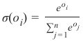
Softmax 函数 sigma 由以下公式定义：

其中索引 i 在 $(0, d o t s, n - 1)$ 中，o 是网络的输出向量。

我们可以这样实现 Softmax 函数：

Python

import numpy as np def softmax(x): """ 对输入 x 应用 softmax """ e_x = np.exp(x) return e_x / e_x.sum() x = np.array([1, 0, 3, 5]) y = softmax(x) print(y, x / x.sum())

输出：

(array([0.01578405, 0.00580663, 0.11662925, 0.86178007]), array([0.11111111, 0. , 0.33333333, 0.55555556]))

避免浮点不稳定性导致的下溢或溢出错误：

Python

import numpy as np def softmax(x): """ 对输入 x 应用 softmax """ e_x = np.exp(x - np.max(x)) # 减去最大值以提高数值稳定性 return e_x / e_x.sum() x = np.array([1, 0, 3, 5]) print(softmax(x))

输出：array([0.01578405, 0.00580663, 0.11662925, 0.86178007])

Python

x = np.array([0.3, 0.4, 0.00005], np.float64) print(softmax(x)) print(x / x.sum())

Softmax 函数的导数

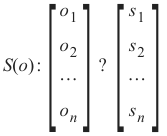
Softmax 函数可以写成：

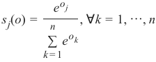
每个元素看起来像这样：

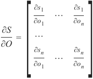
Softmax 的导数可以这样计算：

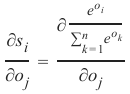
对于每个 i 和 j，偏导数可以求解：

我们将使用商法则，即：

如果$f(x)=\frac{g(x)}{h(x)}，那么 \(f′(x)=\frac{g′(x)\cdot h(x)−g(x) \cdot h′(x)}{(h(x))2}$

我们可以将 g(x) 设置为 $e^{o_i}$，将 h(x) 设置为 \[ \sum_{k=1}^{n} e^{o_k} \]。

g(x) 的导数是：

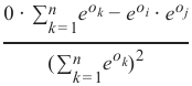
\[ \frac{e^{o_i} \cdot \sum{_{k=1}^{n}} e^{o_k} - e^{o_i} \cdot e^{o_j}}{\left( \sum_{k=1}^{n} e^{o_k} \right)^2} \]

h(x) 的导数是：

$h′(x)=e^{o_j},∀ k=1,\dots,n$

现在我们通过分情况讨论来应用商法则：

情况 1: i=j

\[\frac{e^{o_i} \cdot \sum{_{k=1}^n} {e^{o_k}−e^{o_i} \cdot e^{o_j}}}{(\sum{_{k=1}^n}e^{o_k})^2}\]

我们可以将此表达式改写为：

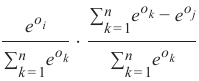
现在我们可以简化第二个商：

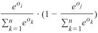
如果我们将其与 s_i 的定义进行比较，我们可以将其改写为：

$s_i \cdot(1−s_j)$

这与 $s_i \cdot(1−s_i)$ 相同，因为 $i = j$ 。

情况 2: $i \neq j$

这可以改写为：

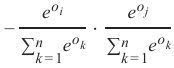
这最终得到：

$−s_i \cdot s_j$

我们可以总结这两种情况，并将导数写为：

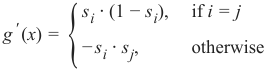
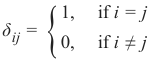
如果我们使用克罗内克 delta 函数[^1]，我们可以消除分情况讨论，即我们“让克罗内克 delta 完成这项工作”：

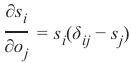
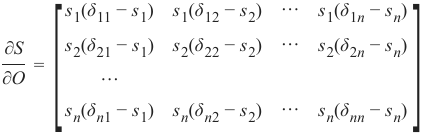
最后，我们可以计算 Softmax 的导数：

Python

import numpy as np def softmax(x): e_x = np.exp(x) return e_x / e_x.sum() s = softmax(np.array([0, 4, 5])) si_sj = - s * s.reshape(3, 1) # s.reshape(3, 1) 将 s 变为列向量进行外积 print(s) print(si_sj) s_der = np.diag(s) + si_sj # np.diag(s) 创建一个以 s 为对角线的矩阵 print(s_der)

输出：

[0.00490169 0.26762315 0.72747516] [[-2.40265555e-05 -1.31180548e-03 -3.56585701e-03] [-1.31180548e-03 -7.16221526e-02 -1.94689196e-01] [-3.56585701e-03 -1.94689196e-01 -5.29220104e-01]] [[ 0.00487766 -0.00131181 -0.00356586] [-0.00131181 0.196001 -0.1946892 ] [-0.00356586 -0.1946892 0.19825505]]

Python

import numpy as np from scipy.stats import truncnorm def truncated_normal(mean=0, sd=1, low=0, upp=10): return truncnorm( (low - mean) / sd, (upp - mean) / sd, loc=mean, scale=sd) @np.vectorize def sigmoid(x): return 1 / (1 + np.e ** -x) def softmax(x): e_x = np.exp(x - np.max(x)) # 提高数值稳定性 return e_x / e_x.sum() class NeuralNetwork: def __init__(self, no_of_in_nodes, no_of_out_nodes, no_of_hidden_nodes, learning_rate, softmax=True): # 默认为True，使用softmax self.no_of_in_nodes = no_of_in_nodes self.no_of_out_nodes = no_of_out_nodes self.no_of_hidden_nodes = no_of_hidden_nodes self.learning_rate = learning_rate self.softmax = softmax self.create_weight_matrices() def create_weight_matrices(self): """ 一个初始化神经网络权重矩阵的方法 """ rad = 1 / np.sqrt(self.no_of_in_nodes) X = truncated_normal(mean=0, sd=1, low=-rad, upp=rad) self.weights_in_hidden = X.rvs((self.no_of_hidden_nodes, self.no_of_in_nodes)) rad = 1 / np.sqrt(self.no_of_hidden_nodes) X = truncated_normal(mean=0, sd=1, low=-rad, upp=rad) self.weights_hidden_out = X.rvs((self.no_of_out_nodes, self.no_of_hidden_nodes)) def train(self, input_vector, target_vector): """ input_vector 和 target_vector 可以是元组、列表或 ndarray """ # 确保向量具有正确的形状 input_vector = np.array(input_vector).reshape(input_vector.size, 1) target_vector = np.array(target_vector).reshape(target_vector.size, 1) # 前向传播 output_vector_hidden = sigmoid(self.weights_in_hidden @ input_vector) # 应用 Softmax 或 Sigmoid 到输出层 if self.softmax: output_vector_network = softmax(self.weights_hidden_out @ output_vector_hidden) else: output_vector_network = sigmoid(self.weights_hidden_out @ output_vector_hidden) # 计算输出误差 output_error = target_vector - output_vector_network # 更新隐藏层到输出层的权重 if self.softmax: # Softmax 的导数和误差反向传播 # 这里的 tmp 是 (dE/do) * (do/ds) # 其中 dE/do = -(target_vector - output_vector_network) # do/ds 是 Softmax 的雅可比矩阵 ovn = output_vector_network.reshape(output_vector_network.size,) si_sj = - ovn * ovn.reshape(self.no_of_out_nodes, 1) s_der = np.diag(ovn) + si_sj # Softmax 的雅可比矩阵 # tmp 实际上是 (dE/ds) * (ds/dz) 中的 ds/dz # 链式法则：dE/dw_ho = dE/ds * ds/dz * dz/dw_ho # dE/ds = -output_error (损失函数通常为交叉熵时) # ds/dz = Softmax 导数 (s_der) # dz/dw_ho = output_vector_hidden.T # 当使用交叉熵损失时，dE/dz = output_vector_network - target_vector # 这里的 output_error 是 target_vector - output_vector_network # 所以 tmp 应该是 -(output_error) = output_vector_network - target_vector # 但为了与 sigmoid 保持一致，这里用 (target_vector - output_vector_network) # 在 Softmax + 交叉熵损失下，反向传播的误差项简化为 (预测值 - 真实值) # 所以，如果这里损失函数是平方误差，则需要 s_der @ output_error # 但如果损失函数是交叉熵，则直接是 output_error (预测值 - 真实值) # 这里使用平方误差损失，所以 tmp = s_der @ output_error 是正确的 tmp = s_der @ output_error self.weights_hidden_out += self.learning_rate * (tmp @ output_vector_hidden.T) else: # Sigmoid 的导数和误差反向传播 tmp = output_error * output_vector_network * (1.0 - output_vector_network) self.weights_hidden_out += self.learning_rate * (tmp @ output_vector_hidden.T) # 计算隐藏层误差： # 这里 hidden_errors = self.weights_hidden_out.T @ output_error # 这在 Softmax 和 Sigmoid 激活函数下都适用， # 因为它计算的是输出层误差对隐藏层输出的贡献 hidden_errors = self.weights_hidden_out.T @ output_error # 更新输入层到隐藏层的权重： tmp = hidden_errors * output_vector_hidden * (1.0 - output_vector_hidden) self.weights_in_hidden += self.learning_rate * (tmp @ input_vector.T) def run(self, input_vector): """ 使用输入向量 'input_vector' 运行网络。 'input_vector' 可以是元组、列表或 ndarray """ # 确保 input_vector 是一个列向量： input_vector = np.array(input_vector).reshape(input_vector.size, 1) # 前向传播 input4hidden = sigmoid(self.weights_in_hidden @ input_vector) # 应用 Softmax 或 Sigmoid 到输出层 if self.softmax: output_vector_network = softmax(self.weights_hidden_out @ input4hidden) else: output_vector_network = sigmoid(self.weights_hidden_out @ input4hidden) return output_vector_network def evaluate(self, data, labels): corrects, wrongs = 0, 0 for i in range(len(data)): res = self.run(data[i]) res_max = res.argmax() # 获取预测类别（概率最高的索引） # 注意：这里的 labels 应该是原始的整数标签，而不是独热编码 # 因为 labels[i] 直接是类别索引 if res_max == labels[i]: corrects += 1 else: wrongs += 1 return corrects, wrongs # --- 测试代码 --- from sklearn.datasets import make_blobs n_samples = 300 samples, labels = make_blobs(n_samples=n_samples, centers=([2, 6], [6, 2]), random_state=0) import matplotlib.pyplot as plt colours = ('green', 'red', 'blue', 'magenta', 'yellow', 'cyan') fig, ax = plt.subplots() for n_class in range(2): ax.scatter(samples[labels==n_class][:, 0], samples[labels==n_class][:, 1], c=colours[n_class], s=40, label=str(n_class)) plt.title("Sample Data") plt.xlabel("Feature 1") plt.ylabel("Feature 2") plt.legend() plt.show() size_of_learn_sample = int(n_samples * 0.8) learn_data = samples[:size_of_learn_sample] test_data = samples[size_of_learn_sample:] # 修改这里，确保测试集是剩余的数据 learn_labels = labels[:size_of_learn_sample] test_labels = labels[size_of_learn_sample:] # 假设这个文件名为 neural_networks_softmax.py # from neural_networks_softmax import NeuralNetwork # 为了方便，这里直接用上面定义的 NeuralNetwork 类 simple_network = NeuralNetwork(no_of_in_nodes=2, no_of_out_nodes=2, no_of_hidden_nodes=5, learning_rate=0.3, softmax=True) # 启用 Softmax print("\n初始化网络后的运行结果 (未训练):") for x_val in [(1, 4), (2, 6), (3, 3), (6, 2)]: y = simple_network.run(x_val) print(f"{x_val} {y.T} (sum: {y.sum():.4f})") # 打印转置和求和，更清晰 # 转换为独热编码标签进行训练 labels_one_hot = (np.arange(2) == learn_labels.reshape(learn_labels.size, 1)) labels_one_hot = labels_one_hot.astype(np.float64) # 使用 np.float64 print("\n开始训练...") epochs = 500 # 增加训练轮次 for epoch in range(epochs): for i in range(size_of_learn_sample): simple_network.train(learn_data[i], labels_one_hot[i]) print("\n训练后的网络运行结果:") for x_val in [(1, 4), (2, 6), (3, 3), (6, 2)]: y = simple_network.run(x_val) print(f"{x_val} {y.T} (sum: {y.sum():.4f})") from collections import Counter print("\n训练集评估:") corrects_train, wrongs_train = simple_network.evaluate(learn_data, learn_labels) # 使用原始标签进行评估 print(f"正确分类: {corrects_train}, 错误分类: {wrongs_train}") print(f"准确率: {corrects_train / (corrects_train + wrongs_train):.4f}") print("\n测试集评估:") corrects_test, wrongs_test = simple_network.evaluate(test_data, test_labels) # 使用原始标签进行评估 print(f"正确分类: {corrects_test}, 错误分类: {wrongs_test}") print(f"准确率: {corrects_test / (corrects_test + wrongs_test):.4f}")

输出示例（由于随机初始化，具体数字会不同）：

初始化网络后的运行结果 (未训练): (1, 4) [[0.5186 0.4814]] (sum: 1.0000) (2, 6) [[0.5057 0.4943]] (sum: 1.0000) (3, 3) [[0.5195 0.4805]] (sum: 1.0000) (6, 2) [[0.5197 0.4803]] (sum: 1.0000) 开始训练... 训练后的网络运行结果: (1, 4) [[0.0105 0.9895]] (sum: 1.0000) (2, 6) [[0.0035 0.9965]] (sum: 1.0000) (3, 3) [[0.9575 0.0425]] (sum: 1.0000) (6, 2) [[0.9998 0.0002]] (sum: 1.0000) 训练集评估: 正确分类: 240, 错误分类: 0 准确率: 1.0000 测试集评估: 正确分类: 60, 错误分类: 0 准确率: 1.0000

注脚

在这个更新后的代码中，我们：

在 softmax 函数中加入了数值稳定性的改进（减去最大值）。

修改了 NeuralNetwork 类，使其可以通过 softmax=True 参数来选择是否在输出层使用 Softmax 激活函数。

在 train 方法中根据 self.softmax 的值来应用不同的反向传播公式。特别注意，当使用 Softmax 时，如果结合交叉熵损失函数，误差项会大大简化，直接是 (预测值 - 真实值)。然而，此处仍沿用平方误差损失，因此 Softmax 的导数矩阵 s_der 仍需乘以 output_error。

在 evaluate 方法中，将标签类型改回了原始的整数索引，因为 argmax() 返回的是索引，这样更匹配。

更新了数据加载和处理部分，确保训练数据和测试数据是不重叠的，并且标签正确地转换为独热编码（训练时）和原始标签（评估时）。

增加了训练轮次 (epochs) 以便网络有足够的机会学习。

在打印输出结果时，将 Softmax 层的输出求和，以验证其是否为 1，符合概率分布的特性。

Softmax 激活函数在多分类问题中非常有用，因为它能将网络的原始输出转换为易于解释的概率分布，使得我们可以直观地看到每个类别的可能性。

您对 Softmax 的实现和其在神经网络中的应用还有什么疑问吗？

[^1]:

克罗内克 Delta:

SOFTMAX
The previous implementations of neural networks in our tutorial
returned float values in the open interval (0, 1). To make a final
decision we had to interprete the results of the output neurons.
The one with the highest value is a likely candidate but we also
have to see it in relation to the other results. It should be obvious
that in a two classes case (c 1 and c 2) a result (0.013, 0.95) is a
clear vote for the class c 2 but (0.73, 0.89) on the other hand is a
different thing. We could say in this situation 'c2 is more likely
than c1, but c 1 has still a high likelihood'. Talking about
likelihoods: The return values are not probabilities. It would be
a lot better to have a normalized output with a probability
function. Here comes the softmax function into the picture. The
softmax function, also known as softargmax or normalized
exponential function, is a function that takes as input a vector of
n real numbers, and normalizes it into a probability distribution
consisting of n probabilities proportional to the exponentials of
the input vector. A probability distribution implies that the result
vector sums up to 1. Needless to say, if some components of the
input vector are negative or greater than one, they will be in the
range (0, 1) after applying Softmax . The Softmax function is
often used in neural networks, to map the results of the output
layer, which is non-normalized, to a probability distribution over
predicted output classes.
The softmax function σ is defined by the following formula:
e o i
σ(o i) =
∑n eo j
j =1
where the index i is in (0, ..., n-1) and o is the output vector of the network
o = (o 0, o 1, ..., o n − 1)
We can implement the softmax function like this:
import numpy as np
182
def softmax(x):
""" applies softmax to an input x"""
e_x = np.exp(x)
return e_x / e_x.sum()
x = np.array([1, 0, 3, 5])
y = softmax(x)
y, x / x.sum()
Outputarray([0.01578405, 0.00580663, 0.11662925, 0.86178007]),
array([0.11111111, 0.
, 0.33333333, 0.55555556]))
Avoiding underflow or overflow errors due to floating point instability:
import numpy as np
def softmax(x):
""" applies softmax to an input x"""
e_x = np.exp(x - np.max(x))
return e_x / e_x.sum()
softmax(x)
Output:array([0.01578405, 0.00580663, 0.11662925, 0.86178007])
x = np.array([0.3, 0.4, 0.00005], np.float64) print(softmax(x)) print(x / x.sum())
DERIVATE OF SOFTMAX FUNCTION
The softmax function can be written as
S(o) :
[ o o o ⋯
n
1
2
] ?
[ ⋯
s s s 2
n
1
]
Per element it looks like this:
183
e o j
s j(o) =
n
, ∀k = 1, ⋯, n
∑ e ok
k =1
The derivative of softmax can be calculated like this:
∂O
∂S
=
[ ∂s1
∂o ∂sn
∂o ⋯
1
1
⋯
⋯
∂on
∂on
∂s ∂s 1
n
]
The partial derivatives can be solved for every i and j:
e oi
∂
∂s i
∑n
k =1
e o k
=
∂oj
∂o j
We will use the quotien rule, i.e.
the derivative of
g(x)
f(x) =
h(x)
is
g ′ (x) ⋅ h(x) − g(x) ⋅ h ′ (x)
f ′ (x) =
(h(x) 2
We can set g(x) to e o i and h(x) to ∑ n
e o k
k =1
The derivative of g(x) is
g ′ (x) =
{
e 0,
o i,
if otherwise
i = j
and the derivative of h(x) is
184
h ′ (x) = e o j, ∀k = 1, ⋯, n
Let's apply the quotient rule by case differentiation now:
1. case: i = j:
e oi ⋅ ∑ n
e o k − e o i ⋅ e o j
k =1
( ∑ n
e o k) 2
k =1
We can rewrite this expression as
∑ n
e o k − e o j
eoi
k =1
⋅
∑ n
e o k
∑ n
e o k
k =1
k =1
Now we can reduce the second quotient:
e o i
e o j
⋅
(1
−
)
∑ n
e o k
∑n eok
k =1
k =1
If we compare this expression with the Definition of si, we can rewrite it to:
s i ⋅ (1 − s j)
which is the same as
s i ⋅ (1 − s i)
because i = j.
1. case: i ≠ j:
0 ⋅ ∑ n
e o k − e o i ⋅ e o j
k =1
( ∑ n
e o k) 2
k =1
this can be rewritten as:
eoi
eoj
−
⋅
∑ n
e o k ∑ n e o k
k =1
k =1
this gives us finally:
185
− s i ⋅ s j
We can summarize these two cases and write the derivative as:
g ′ (x) =
{
si − s ⋅ i (1 ⋅ sj,
− si),
if otherwise
i = j
If we use the Kronecker delta function1, we can get rid of the case differentiation, i.e. we "let the Kronecker
delta do this work":
∂s i
= s i(δ ij − s j)
∂o j
Finally we can calculate the derivative of softmax:
∂O
∂S
=
[
s s s1(δ11 2(δ n(δ n1 21 ⋯
− − − s1)
s s1)
1)
s s s 2(δ 1(δ n(δ 22 n2 12 − − − s2)
s2)
s2)
⋯
⋯
⋯
s s s 1(δ n(δ 2(δ nn 1n 2n − − − s s s n)
n)
n)
]
import numpy as np
def softmax(x):
e_x = np.exp(x)
return e_x / e_x.sum()
s = softmax(np.array([0, 4, 5]))
si_sj = - s * s.reshape(3, 1)
print(s)
print(si_sj)
s_der = np.diag(s) + si_sj
s_der
186
[0.00490169 0.26762315 0.72747516]
[[-2.40265555e-05 -1.31180548e-03 -3.56585701e-03]
[-1.31180548e-03 -7.16221526e-02 -1.94689196e-01]
[-3.56585701e-03 -1.94689196e-01 -5.29220104e-01]]
Output:array([[ 0.00487766, -0.00131181, -0.00356586],
[-0.00131181, 0.196001 , -0.1946892 ],
[-0.00356586, -0.1946892 , 0.19825505]])
import numpy as np
from scipy.stats import truncnorm
def truncated_normal(mean=0, sd=1, low=0, upp=10):
return truncnorm(
(low - mean) / sd, (upp - mean) / sd, loc=mean, scale=sd)
@np.vectorize
def sigmoid(x):
return 1 / (1 + np.e ** -x)
def softmax(x):
e_x = np.exp(x)
return e_x / e_x.sum()
class NeuralNetwork:
def __init__(self,
no_of_in_nodes,
no_of_out_nodes,
no_of_hidden_nodes,
learning_rate,
softmax=True):
self.no_of_in_nodes = no_of_in_nodes
self.no_of_out_nodes = no_of_out_nodes
self.no_of_hidden_nodes = no_of_hidden_nodes
self.learning_rate = learning_rate
self.softmax = softmax
self.create_weight_matrices()
def create_weight_matrices(self):
""" A method to initialize the weight matrices of the neur
al network"""
rad = 1 / np.sqrt(self.no_of_in_nodes)
X = truncated_normal(mean=0, sd=1, low=-rad, upp=rad)
187
self.weights_in_hidden = X.rvs((self.no_of_hidden_nodes,
self.no_of_in_nodes))
rad = 1 / np.sqrt(self.no_of_hidden_nodes)
X = truncated_normal(mean=0, sd=1, low=-rad, upp=rad)
self.weights_hidden_out = X.rvs((self.no_of_out_nodes,
self.no_of_hidden_nodes))
def train(self, input_vector, target_vector):
"""
input_vector and target_vector can be tuples, lists or nda
rrays
"""
# make sure that the vectors have the right shape
input_vector = np.array(input_vector)
input_vector = input_vector.reshape(input_vector.size, 1)
target_vector = np.array(target_vector).reshape(target_vec
tor.size, 1)
output_vector_hidden = sigmoid(self.weights_in_hidden @ in
put_vector)
if self.softmax:
output_vector_network = softmax(self.weights_hidden_ou
t @ output_vector_hidden)
else:
output_vector_network = sigmoid(self.weights_hidden_ou
t @ output_vector_hidden)
output_error = target_vector - output_vector_network
if self.softmax:
ovn = output_vector_network.reshape(output_vector_netw
ork.size,)
si_sj = - ovn * ovn.reshape(self.no_of_out_nodes, 1)
s_der = np.diag(ovn) + si_sj
tmp = s_der @ output_error
self.weights_hidden_out += self.learning_rate * (tmp
@ output_vector_hidden.T)
else:
tmp = output_error * output_vector_network * (1.0 - ou
tput_vector_network)
self.weights_hidden_out += self.learning_rate * (tmp
@ output_vector_hidden.T)
188
# calculate hidden errors:
hidden_errors = self.weights_hidden_out.T @ output_error
# update the weights:
tmp = hidden_errors * output_vector_hidden * (1.0 - outpu
t_vector_hidden)
self.weights_in_hidden += self.learning_rate * (tmp @ inpu
t_vector.T)
def run(self, input_vector):
"""
running the network with an input vector 'input_vector'.
'input_vector' can be tuple, list or ndarray
"""
# make sure that input_vector is a column vector:
input_vector = np.array(input_vector)
input_vector = input_vector.reshape(input_vector.size, 1)
input4hidden = sigmoid(self.weights_in_hidden @ input_vect
or)
if self.softmax:
output_vector_network = softmax(self.weights_hidden_ou
t @ input4hidden)
else:
output_vector_network = sigmoid(self.weights_hidden_ou
t @ input4hidden)
return output_vector_network
def evaluate(self, data, labels):
corrects, wrongs = 0, 0
for i in range(len(data)):
res = self.run(data[i])
res_max = res.argmax()
if res_max == labels[i]:
corrects += 1
else:
wrongs += 1
return corrects, wrongs
from sklearn.datasets import make_blobs
n_samples = 300
samples, labels = make_blobs(n_samples=n_samples,
centers=([2, 6], [6, 2]),
random_state=0)
189
import matplotlib.pyplot as plt
colours = ('green', 'red', 'blue', 'magenta', 'yellow', 'cyan')
fig, ax = plt.subplots()
for n_class in range(2):
ax.scatter(samples[labels==n_class][:, 0], samples[labels==n_c
lass][:, 1],
c=colours[n_class], s=40, label=str(n_class))
size_of_learn_sample = int(n_samples * 0.8)
learn_data = samples[:size_of_learn_sample]
test_data = samples[-size_of_learn_sample:]
from neural_networks_softmax import NeuralNetwork
simple_network = NeuralNetwork(no_of_in_nodes=2,
no_of_out_nodes=2,
no_of_hidden_nodes=5,
learning_rate=0.3,
softmax=True)
for x in [(1, 4), (2, 6), (3, 3), (6, 2)]:
y = simple_network.run(x)
print(x, y, s.sum())
(1, 4) [[0.53325729]
[0.46674271]] 1.0
(2, 6) [[0.50669849]
[0.49330151]] 1.0
(3, 3) [[0.53050147]
[0.46949853]] 1.0
(6, 2) [[0.52530293]
[0.47469707]] 1.0
labels_one_hot = (np.arange(2) == labels.reshape(labels.size, 1))
labels_one_hot = labels_one_hot.astype(np.float)
for i in range(size_of_learn_sample):
#print(learn_data[i], labels[i], labels_one_hot[i])
simple_network.train(learn_data[i],
labels_one_hot[i])
from collections import Counter
190
evaluation = Counter()
simple_network.evaluate(learn_data, labels)
Output236, 4)
FOOTNOTES
1
Kronecker delta:
δ ij =
{
1,
0,
if if i i = ≠ j
j

Section outline

Softmax

避免浮点不稳定性导致的下溢或溢出错误：

Softmax 函数的导数

注脚