数字数据集的神经网络(A Neural Network for the Digits Dataset)
章节大纲
-
简介
Python 的 scikit-learn 模块包含一个手写数字数据集。正如我们在《数据表示和可视化》一章中所示,这只是 scikit-learn 提供的众多数据集之一。在本机器学习教程的这一章中,我们将演示如何为数字数据集创建神经网络以识别这些数字。本示例旨在通过实际操作来补充我们之前章节的理论介绍。您将看到,完成实际的分类和识别任务几乎不需要任何 Python 代码。
我们首先加载数字数据:
Pythonfrom sklearn.datasets import load_digits digits = load_digits()我们可以使用
keys方法概览数据集中包含的内容:Pythondigits.keys()Output:
dict_keys(['data', 'target', 'frame', 'feature_names', 'target_names', 'images', 'DESCR'])digits 数据集包含 1797 张图像,每张图像包含 64 个特征,这些特征对应于像素:
Pythonn_samples, n_features = digits.data.shape print((n_samples, n_features))Output:
(1797, 64)Pythonprint(digits.data[0])Output:
[ 0. 0. 5. 13. 9. 1. 0. 0. 0. 0. 13. 15. 10. 15. 5. 0. 0. 3. 15. 2. 0. 11. 8. 0. 0. 4. 12. 0. 0. 8. 8. 0. 0. 5. 8. 0. 0. 9. 8. 0. 0. 4. 11. 0. 1. 12. 7. 0. 0. 2. 14. 5. 1. 0. 12. 0. 0. 0. 0. 6. 13. 10. 0. 0. 0.]Pythonprint(digits.target)Output:
[0 1 2 ... 8 9 8]数据也可通过
digits.images获取。这是以 8 行 8 列形式表示的原始图像数据。对于“data”,一张图像对应一个长度为 64 的一维 Numpy 数组;而“images”表示形式包含形状为 (8, 8) 的二维 numpy 数组。
Pythonprint("Shape of an item: ", digits.data[0].shape) print("Data type of an item: ", type(digits.data[0])) print("Shape of an item: ", digits.images[0].shape) print("Data tpye of an item: ", type(digits.images[0]))Output:
Shape of an item: (64,) Data type of an item: <class 'numpy.ndarray'> Shape of an item: (8, 8) Data tpye of an item: <class 'numpy.ndarray'>让我们将数据可视化:
Pythonimport matplotlib.pyplot as plt plt.imshow(digits.images[0], cmap='binary') plt.show()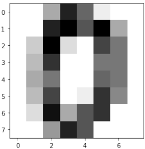
让我们结合它们的标签可视化更多数字:
Pythonimport matplotlib.pyplot as plt # 设置图像 fig = plt.figure(figsize=(6, 6)) # 图像尺寸(英寸) fig.subplots_adjust(left=0, right=1, bottom=0, top=1, hspace=0.05, wspace=0.05) # 绘制数字:每张图像为 8x8 像素 for i in range(64): ax = fig.add_subplot(8, 8, i + 1, xticks=[], yticks=[]) ax.imshow(digits.images[i], cmap=plt.cm.binary, interpolation='nearest') # 用目标值标记图像 ax.text(0, 7, str(digits.target[i])) plt.show() # 显示图表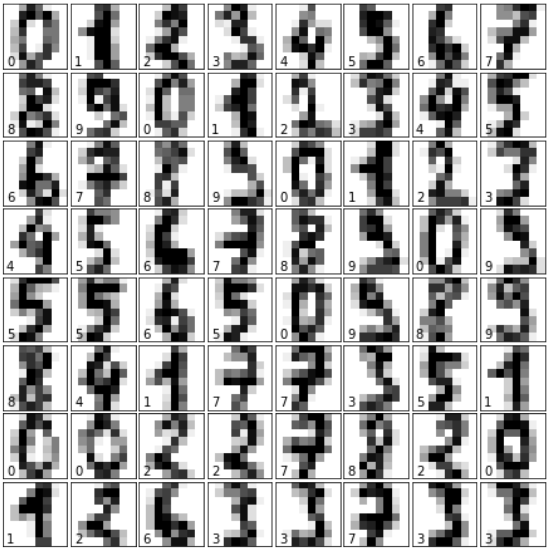 Python
import matplotlib.pyplot as plt # 设置图像 fig = plt.figure(figsize=(6, 6)) # 图像尺寸(英寸) fig.subplots_adjust(left=0, right=1, bottom=0, top=1, hspace=0.05, wspace=0.05) # 绘制数字:每张图像为 8x8 像素 for i in range(144): ax = fig.add_subplot(12, 12, i + 1, xticks=[], yticks=[]) ax.imshow(digits.images[i], cmap=plt.cm.binary, interpolation='nearest') # 用目标值标记图像 #ax.text(0, 7, str(digits.target[i])) # 此行被注释掉 plt.show() # 显示图表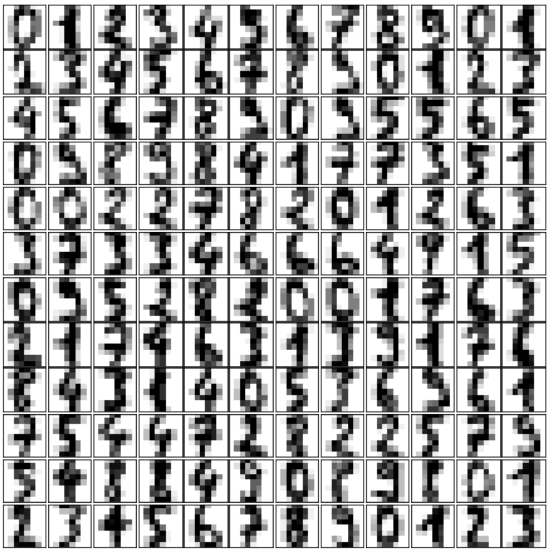 Python
from sklearn.model_selection import train_test_split res = train_test_split(digits.data, digits.target, train_size=0.8, test_size=0.2, random_state=1) train_data, test_data, train_labels, test_labels = res from sklearn.neural_network import MLPClassifier mlp = MLPClassifier(hidden_layer_sizes=(5,), activation='logistic', alpha=1e-4, solver='sgd', tol=1e-4, random_state=1, learning_rate_init=.3, verbose=True)Pythonmlp.fit(train_data, train_labels)Output:
Iteration 1, loss = 2.25145782 Iteration 2, loss = 1.97730357 Iteration 3, loss = 1.66620880 Iteration 4, loss = 1.41353830 Iteration 5, loss = 1.29575643 Iteration 6, loss = 1.06663573 Iteration 7, loss = 0.95558862 Iteration 8, loss = 0.94767318 Iteration 9, loss = 0.95242867 Iteration 10, loss = 0.83577430 Iteration 11, loss = 0.74541414 Iteration 12, loss = 0.72011102 Iteration 13, loss = 0.70790928 Iteration 14, loss = 0.69425700 Iteration 15, loss = 0.74458525 Iteration 16, loss = 0.67779333 Iteration 17, loss = 0.69691846 Iteration 18, loss = 0.67844516 Iteration 19, loss = 0.68164743 Iteration 20, loss = 0.68435917 Iteration 21, loss = 0.61988051 Iteration 22, loss = 0.61362164 Iteration 23, loss = 0.56615517 Iteration 24, loss = 0.61323269 Iteration 25, loss = 0.56979209 Iteration 26, loss = 0.58189564 Iteration 27, loss = 0.50692207 Iteration 28, loss = 0.65956191 Iteration 29, loss = 0.53736180 Iteration 30, loss = 0.66437126 Iteration 31, loss = 0.56201738 Iteration 32, loss = 0.85347048 Iteration 33, loss = 0.63673358 Iteration 34, loss = 0.69769079 Iteration 35, loss = 0.62714187 Iteration 36, loss = 0.56914708 Iteration 37, loss = 1.05660379 Iteration 38, loss = 0.66966105 Training loss did not improve more than tol=0.000100 for 10 consecutive epochs. Stopping.Output:
MLPClassifier(activation='logistic', alpha=0.0001, batch_size='auto', beta_1=0.9, beta_2=0.999, early_stopping=False, epsilon=1e-08, hidden_layer_sizes=(5,), learning_rate='constant', learning_rate_init=0.3, max_iter=200, momentum=0.9, n_iter_no_change=10, nesterovs_momentum=True, power_t=0.5, random_state=1, shuffle=True, solver='sgd', tol=0.0001, validation_fraction=0.1, verbose=True, warm_start=False)Pythonpredictions = mlp.predict(test_data) print(predictions[:25] , test_labels[:25])Output:
(array([1, 5, 0, 7, 7, 0, 6, 1, 5, 4, 9, 2, 7, 8, 4, 1, 7, 3, 7, 4, 7, 4, 8, 6, 0]), array([1, 5, 0, 7, 1, 0, 6, 1, 5, 4, 9, 2, 7, 8, 4, 6, 9, 3, 7, 4, 7, 1, 8, 6, 0]))Pythonfrom sklearn.metrics import accuracy_score print(accuracy_score(test_labels, predictions))Output:
0.725Pythonfor i in range(5, 30): mlp = MLPClassifier(hidden_layer_sizes=(i,), activation='logistic', random_state=1, alpha=1e-4, solver='sgd', tol=1e-4, learning_rate_init=.3, verbose=False) mlp.fit(train_data, train_labels) predictions = mlp.predict(test_data) acc_score = accuracy_score(test_labels, predictions) print(i, acc_score)Output:
5 0.725 6 0.37222222222222223 7 0.8166666666666667 8 0.8666666666666667 9 0.8805555555555555 10 0.925 11 0.9388888888888889 12 0.9388888888888889 13 0.9388888888888889 14 0.9527777777777777 15 0.9305555555555556 16 0.95 17 0.8916666666666667 18 0.8638888888888889 /home/bernd/anaconda3/lib/python3.7/site-packages/sklearn/neural_network/multilayer_perceptron.py:562: ConvergenceWarning: Stochastic Optimizer: Maximum iterations (200) reached and the optimization hasn't converged yet. % self.max_iter, ConvergenceWarning) 19 0.9555555555555556 20 0.9638888888888889 21 0.9722222222222222 22 0.9611111111111111 23 0.9444444444444444 24 0.9583333333333334 25 0.9305555555555556 26 0.9722222222222222 27 0.9694444444444444 28 0.975 29 0.9611111111111111Pythonfrom sklearn.model_selection import GridSearchCV param_grid = [ { 'activation' : ['identity', 'logistic', 'tanh', 'relu'], 'solver' : ['lbfgs', 'sgd', 'adam'], 'hidden_layer_sizes': [ (1,),(2,),(3,),(4,),(5,),(6,),(7,),(8,),(9,),(10,),(11,), (12,),(13,),(14,),(15,),(16,),(17,),(18,),(19,),(20,),(21,) ] } ]Pythonclf = GridSearchCV(MLPClassifier(), param_grid, cv=3, scoring='accuracy') clf.fit(train_data, train_labels) print("Best parameters set found on development set:") print(clf.best_params_)
INTRODUCTION
The Python module sklear contains a
dataset with handwritten digits. It is just
one of many datasets which sklearn
provides, as we show in our chapter
Representation and Visualization of Data.
In this chapter of our Machine Learning
tutorial we will demonstrate how to create
a neural network for the digits dataset to
recognize these digits. This example is
accompanying the theoretical
introductions of our previous chapters to
give a practical view. You will see that
hardly any Python code is needed to
accomplish the actual classification and
recognition task.
We will first load the digits data:
In [ ]:
from sklearn.datasets imp
ort load_digits
digits = load_digits()
We can get an overview of what is
contained in the dataset with the keys method:
digits.keys()
Output:dict_keys(['data', 'target', 'frame', 'feature_names', 'targe
t_names', 'images', 'DESCR'])
The digits dataset contains 1797 images and each images contains 64 features, which correspond to the pixels:
269
n_samples, n_features = digits.data.shape
print((n_samples, n_features))
(1797, 64)
print(digits.data[0])
[ 0. 0.
5. 13.
9.
1.
0.
0.
0.
0. 13. 15. 10. 15.
5.
0.
0. 3.
15. 2.
0. 11.
8.
0.
0.
4. 12.
0.
0.
8.
8.
0.
0.
5.
8. 0.
0. 9.
8.
0.
0.
4. 11.
0.
1. 12.
7.
0.
0.
2. 14.
5. 1
0. 12.
0. 0.
0.
0.
6. 13. 10.
0.
0.
0.]
print(digits.target)
[0 1 2 ... 8 9 8]
The data is also available at digits.images. This is the raw data of the images in the form of 8 lines and 8
columns.
With "data" an image corresponds to a one-dimensional Numpy array with the length 64, and "images"
representation contains 2-dimensional numpy arrays with the shape (8, 8)
print("Shape of an item: ", digits.data[0].shape)
print("Data type of an item: ", type(digits.data[0]))
print("Shape of an item: ", digits.images[0].shape)
print("Data tpye of an item: ", type(digits.images[0]))
Shape of an item: (64,)
Data type of an item: <class 'numpy.ndarray'>
Shape of an item: (8, 8)
Data tpye of an item: <class 'numpy.ndarray'>
Let's visualize the data:
import matplotlib.pyplot as plt
plt.imshow(digits.images[0], cmap='binary')
plt.show()
270
Let's visualize some more digits combined with their labels:
import matplotlib.pyplot as plt
# set up the figure
fig = plt.figure(figsize=(6, 6)) # figure size in inches
fig.subplots_adjust(left=0, right=1, bottom=0, top=1, hspace=0.0
5, wspace=0.05)
# plot the digits: each image is 8x8 pixels
for i in range(64):
ax = fig.add_subplot(8, 8, i + 1, xticks=[], yticks=[])
ax.imshow(digits.images[i], cmap=plt.cm.binary, interpolatio
n='nearest')
# label the image with the target value
ax.text(0, 7, str(digits.target[i]))
271
import matplotlib.pyplot as plt
# set up the figure
fig = plt.figure(figsize=(6, 6)) # figure size in inches
fig.subplots_adjust(left=0, right=1, bottom=0, top=1, hspace=0.0
5, wspace=0.05)
# plot the digits: each image is 8x8 pixels
for i in range(144):
ax = fig.add_subplot(12, 12, i + 1, xticks=[], yticks=[])
ax.imshow(digits.images[i], cmap=plt.cm.binary, interpolatio
n='nearest')
# label the image with the target value
#ax.text(0, 7, str(digits.target[i]))
272
from sklearn.model_selection import train_test_split
res = train_test_split(digits.data, digits.target,
train_size=0.8,
test_size=0.2,
random_state=1)
train_data, test_data, train_labels, test_labels = res
from sklearn.neural_network import MLPClassifier
mlp = MLPClassifier(hidden_layer_sizes=(5,),
activation='logistic',
alpha=1e-4,
solver='sgd',
tol=1e-4,
random_state=1,
learning_rate_init=.3,
verbose=True)
273
mlp.fit(train_data, train_labels)
274
Iteration 1, loss = 2.25145782
Iteration 2, loss = 1.97730357
Iteration 3, loss = 1.66620880
Iteration 4, loss = 1.41353830
Iteration 5, loss = 1.29575643
Iteration 6, loss = 1.06663573
Iteration 7, loss = 0.95558862
Iteration 8, loss = 0.94767318
Iteration 9, loss = 0.95242867
Iteration 10, loss = 0.83577430
Iteration 11, loss = 0.74541414
Iteration 12, loss = 0.72011102
Iteration 13, loss = 0.70790928
Iteration 14, loss = 0.69425700
Iteration 15, loss = 0.74458525
Iteration 16, loss = 0.67779333
Iteration 17, loss = 0.69691846
Iteration 18, loss = 0.67844516
Iteration 19, loss = 0.68164743
Iteration 20, loss = 0.68435917
Iteration 21, loss = 0.61988051
Iteration 22, loss = 0.61362164
Iteration 23, loss = 0.56615517
Iteration 24, loss = 0.61323269
Iteration 25, loss = 0.56979209
Iteration 26, loss = 0.58189564
Iteration 27, loss = 0.50692207
Iteration 28, loss = 0.65956191
Iteration 29, loss = 0.53736180
Iteration 30, loss = 0.66437126
Iteration 31, loss = 0.56201738
Iteration 32, loss = 0.85347048
Iteration 33, loss = 0.63673358
Iteration 34, loss = 0.69769079
Iteration 35, loss = 0.62714187
Iteration 36, loss = 0.56914708
Iteration 37, loss = 1.05660379
Iteration 38, loss = 0.66966105
Training loss did not improve more than tol=0.000100utive epochs. Stopping.
for 10 consec
275
Output:MLPClassifier(activation='logistic', alpha=0.0001, batch_siz
e='auto',
beta_1=0.9, beta_2=0.999, early_stopping=False, epsilo
n=1e-08,
hidden_layer_sizes=(5,), learning_rate='constant',
learning_rate_init=0.3, max_iter=200, momentum=0.9,
n_iter_no_change=10, nesterovs_momentum=True, powe
r_t=0.5,
random_state=1, shuffle=True, solver='sgd', tol=0.000
1,
validation_fraction=0.1, verbose=True, warm_start=Fals
e)
predictions = mlp.predict(test_data)
predictions[:25] , test_labels[:25]
Outputarray([1, 5, 0, 7, 7, 0, 6, 1, 5, 4, 9, 2, 7, 8, 4, 1, 7,
3, 7, 4, 7, 4,
8, 6, 0]),
array([1, 5, 0, 7, 1, 0, 6, 1, 5, 4, 9, 2, 7, 8, 4, 6, 9,
3, 7, 4, 7, 1,
8, 6, 0]))
from sklearn.metrics import accuracy_score
accuracy_score(test_labels, predictions)
Output:0.725
for i in range(5, 30):
    mlp = MLPClassifier(hidden_layer_sizes=(i,),
    activation='logistic',
    random_state=1,
    alpha=1e-4,
    solver='sgd',
    tol=1e-4,
    learning_rate_init=.3,
    verbose=False)
    mlp.fit(train_data, train_labels)
    predictions = mlp.predict(test_data)
    acc_score = accuracy_score(test_labels, predictions)
    print(i, acc_score)
276
5 0.725
6 0.37222222222222223
7 0.8166666666666667
8 0.8666666666666667
9 0.8805555555555555
10 0.925
11 0.9388888888888889
12 0.9388888888888889
13 0.9388888888888889
14 0.9527777777777777
15 0.9305555555555556
16 0.95
17 0.8916666666666667
18 0.8638888888888889
/home/bernd/anaconda3/lib/python3.7/site-packages/sklearn/neural_n
etwork/multilayer_perceptron.py:562: ConvergenceWarning: Stochasti
c Optimizer: Maximum iterations (200) reached and the optimizatio
n hasn't converged yet.
% self.max_iter, ConvergenceWarning)
19202122232425262728290.9555555555555556
0.9638888888888889
0.9722222222222222
0.9611111111111111
0.9444444444444444
0.9583333333333334
0.9305555555555556
0.9722222222222222
0.9694444444444444
0.975
0.9611111111111111
In [ ]:
In [ ]:
In [ ]:
In [ ]:
from sklearn.model_selection import GridSearchCV
277
param_grid = [
{
'activation' : ['identity', 'logistic', 'tanh', 'rel
u'],
'solver' : ['lbfgs', 'sgd', 'adam'],
'hidden_layer_sizes': [
(1,),(2,),(3,),(4,),(5,),(6,),(7,),(8,),(9,),(10,),(1
1,), (12,),(13,),(14,),(15,),(16,),(17,),(18,),(19,),(20,),(21,)
]
}
]
In [ ]:
clf = GridSearchCV(MLPClassifier(), param_grid, cv=3,
scoring='accuracy')
clf.fit(train_data, train_labels)
print("Best parameters set found on development set:")
print(clf.best_params_)