回归树(Regression Trees)
章节大纲
-
引言 (INTRODUCTION)
在前一章关于分类决策树的内容中,我们介绍了决策树模型的基本概念、如何从零开始用 Python 构建它们,以及如何使用
sklearn预打包的DecisionTreeClassifier方法。我们还介绍了决策树模型的优点和缺点,以及重要的扩展和变体。分类决策树的一个缺点是它们需要一个分类尺度的目标特征,例如weather = {Sunny, Rainy, Overcast, Thunderstorm}。这里出现了一个问题:如果我们的树想要预测房子的价格,给定一些目标特征属性,如房间数量和位置,该怎么办?在这种情况下,目标特征(价格)的值不再是分类尺度的,而是连续的——理论上,一栋房子可以有无限多种不同的价格。
这就是回归树的作用。回归树的原理与分类树相同,但最大的区别在于目标特征值现在可以取无限多个连续尺度的值。因此,现在的任务是预测连续尺度的目标特征 Y 的值,给定一组分类(或连续)尺度的描述性特征 X 的值。
如上所述,构建回归树的原理与创建分类树的方法相同。
我们寻找能最纯粹地分割目标特征值的描述性特征,沿着该描述性特征的值分割数据集,并对每个子数据集重复此过程,直到达到停止标准。如果我们达到停止标准,我们就生成一个叶节点。
然而,有几点发生了变化。
首先,让我们考虑在分类树章节中介绍的用于生成叶节点的停止标准:
-
如果分裂过程导致数据集为空,返回原始数据集的众数目标特征值。
-
如果分裂过程导致数据集中没有剩余特征,返回直接父节点的众数目标特征值。
-
如果分裂过程导致数据集中的目标特征值是纯的,返回该值。
如果我们现在考虑我们新的连续尺度目标特征的属性,我们会发现第三个停止标准不能再使用了,因为目标特征值现在可以取无限多个不同的值。因此,我们极不可能找到纯粹的目标特征值,除非数据集中只剩下一个实例。
简而言之,通常没有纯粹的目标特征值这种东西。
为了解决这个问题,我们将引入一个早期停止标准:如果数据集中实例的数量小于或等于 5,则返回数据集中剩余目标特征值的平均值。
一般来说,在处理回归树时,我们将在叶节点处返回平均目标特征值作为预测。
我们必须进行的第二个改变在考虑分裂过程本身时变得显而易见。
在使用分类树时,我们使用特征的信息增益 (IG) 作为分裂标准。也就是说,具有最大信息增益的特征被用来分割数据集。考虑以下示例,我们只检查一个描述性特征,比如卧室数量,以及房屋成本作为目标特征。
Pythonimport pandas as pd import numpy as np df = pd.DataFrame({'Number_of_Bedrooms':[2,2,4,1,3,1,4,2],'Price_of_Sale':[100000,120000,250000,80000,220000,170000,500000,75000]}) print(df)Output:
   Number_of_Bedrooms  Price_of_Sale
0                   2         100000
1                   2         120000
2                   4         250000
3                   1          80000
4                   3         220000
5                   1         170000
6                   4         500000
7                   2          75000
那么我们如何计算
Number_of_Bedrooms特征的熵呢?如果我们计算加权熵,我们会看到对于 ,我们得到的加权熵为 0。我们得到这个结果是因为数据集中只有一栋房子有 3 间卧室。另一方面,对于 (出现三次),我们将得到 0.59436 的加权熵。
简而言之,由于我们的目标特征是连续尺度的,分类尺度描述性特征的信息增益不再是合适的分裂标准。
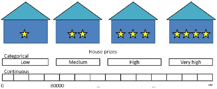
嗯,我们可以转而根据目标特征的值对其进行分类,例如,将房价在 0 美元到 80000 美元之间归类为“低”,80001 美元到 150000 美元之间归类为“中”,150001 美元以上归类为“高”。
我们在这里所做的,是将我们的回归问题转换成了某种分类问题。然而,由于我们希望能够从无限多的可能值(回归)中进行预测,这并不是我们正在寻找的。
让我们回到最初的问题:我们希望有一个分裂标准,它能够以这样一种方式分割数据集:当到达一个树节点时,预测值(我们将预测值定义为该叶节点处实例的平均目标特征值,其中我们将最少 5 个实例定义为早期停止标准)最接近实际值。
事实证明,方差是回归树最常用的分裂标准之一,我们将使用方差作为分裂标准。
这样做的解释是,我们希望寻找那些在沿这些目标特征值分割数据集时,最精确地指向真实目标特征值的特征属性。因此,请看下面的图片。您认为
Number_of_Bedrooms特征的这两种布局中,哪一种能更精确地指向真实销售价格?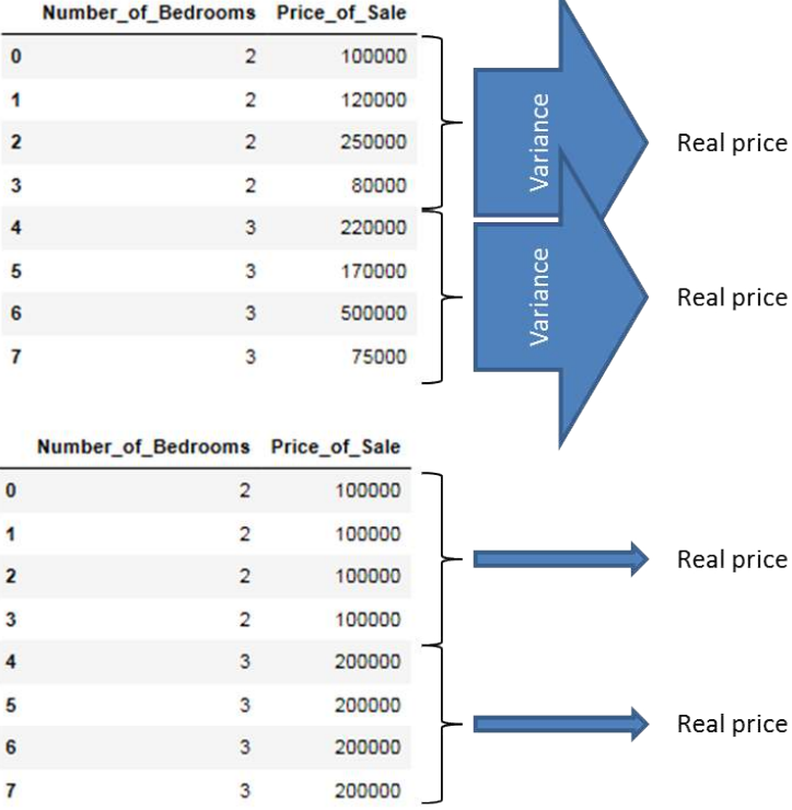
嗯,显然是方差最小的那个!我们将在下一节介绍方差度量背后的数学原理。
目前,我们首先用箭头来表示这些,其中宽箭头表示高方差,细箭头表示低方差。我们可以通过显示描述性特征的每个值对应的目标特征的方差来阐明这一点。正如您所看到的,当我们在沿描述性特征的值分割数据集时,最小化目标特征值方差的特征布局是最精确地指向真实值的特征布局,因此应该用作分裂标准。在创建我们的回归树模型时,我们将使用方差度量来取代信息增益作为分裂标准。
In the previous chapter about
Classification decision Trees we have
introduced the basic concepts underlying
decision tree models, how they can be
build with Python from scratch as well as
using the prepackaged sklearn
DecisionTreeClassifier method. We have
also introduced advantages and
disadvantages of decision tree models as
well as important extensions and
variations. One disadvantage of
Classification decision Trees is that they
need a target feature which is
categorically scaled like for instance
weather = {Sunny, Rainy, Overcast,
Thunderstorm}.
Here arises a problem: What if we want our tree for instance to predict the price of a house given some target
feature attributes like the number of rooms and the location? Here the values of the target feature (prize) are no
longer categorically scaled but are continuous - A house can have, theoretically, a infinite number of different
prices -
Thats where Regression Trees come in. Regression Trees work in principal in the same way as Classification
Trees with the large difference that the target feature values can now take on an infinite number of
continuously scaled values. Hence the task is now to predict the value of a continuously scaled target feature Y
given the values of a set of categorically (or continuously) scaled descriptive features X.
413
As stated above, the principle of building a Regression Tree follows the same approach as the creation of a
Classification Tree.
We search for the descriptive feature which splits the target feature values most purely, divide the dataset
along the values of this descriptive feature and repeat this process for each of the sub datasets until we
accomplish a stopping criteria.If we accomplish a stopping criteria, we grow a leaf node.
Though, a few things changed.
First of all, let us consider the stopping criteria we have introduced in the Classification Tree chapter to grow a
leaf node:
1.2.3.If the splitting process leads to a empty dataset, return the mode target feature value of the
original dataset
If the splitting process leads to a dataset where no features are left, return the mode target feature
value of the direct parent node
If the splitting process leads to a dataset where the target feature values are pure, return this
value
If we now consider the property of our new continuously scaled target feature we mention that the third
stopping criteria can no longer be used since the target feature values can now take on an infinite number of
different values. Consequently, it is most likely that we will not find pure target feature values until there is
only one instance left in the dataset.
To make a long story short, there is in general nothing like pure target feature values.
To address this issue, we will introduce an early stopping criteria that returns the average value of the target
feature values left in the dataset if the number of instances in the dataset is ≤ 5.
In general, while handling with Regression Trees we will return the average target feature values as prediction
at a leaf node.
The second change we have to make becomes apparent when we consider the splitting process itself.
While working with Classification Trees we used the Information Gain (IG) of a feature as splitting criteria.
That is, the feature with the largest IG was used to split the dataset on. Consider the following example where
we examine only one descriptive feature, lets say the number of bedrooms, and the costs of the house as target
feature.
import pandas as pd
import numpy as np
df = pd.DataFrame({'Number_of_Bedrooms':[2,2,4,1,3,1,4,2],'Price_o
f_Sale':[100000,120000,250000,80000,220000,170000,500000,75000]})
df
414
Output:
Number_of_Bedrooms
Price_of_Sale
0
2
100000
1
2
120000
2
4
250000
3
1
80000
4
3
220000
5
1
170000
6
4
500000
7
2
75000
Now how would we calculate the entropy of the Number_of_Bedrooms feature?
| D |
Number of Bedrooms = jH(Number of Bedrooms) = ∑j ∈ Number of Bedrooms ∗ (
| D |
∗ ( ∑ k ∈ Price of Sale ∗ ( − P(k | j) ∗ log2(P(k | j))
If we calculate the weighted entropies, we see that for j = 3, we get a weighted entropy of 0. We get this result
because there is only one house in the dataset with 3 bedrooms. On the other hand, for j = 2 (occurs three
times) we will get a weighted entropy of 0.59436.
To make a long story short, since our target feature is continuously scaled, the IGs of the categorically scaled
descriptive features are no longer appropriate splitting criteria.
Well, we could instead categorize the target feature along its values where for instance housing prices between
$0 and $80000 are categorized as low, between $80001 and $150000 as middle and > $150001
as high.
What we have done here is converting our regression problem into kind of a classification problem. Though,
since we want to be able to make predictions from a infinite number of possible values (regression) this is not
what we are looking for.
Lets come back to our initial issue: We want to have a splitting criteria which allows us to split the dataset in
such a way that when arriving a tree node, the predicted value (we defined the predicted value as the mean
target feature value of the instances at this leaf node where we defined the minimum number of 5 instances as
early stopping criteria) is closest to the actual value.
It turns out that the variance is one of the most commonly used splitting criteria for regression trees where we
will use the variance as splitting criteria.
The explanation therefore is, that we want to search for the feature attributes which most exactly point to the
415
real target feature values when splitting the dataset along the values of these target features. Therefore,
examine the following picture. What do you think which of those two layouts of the Number_of_Bedrooms
feature points more exactly to the real sales prize?
Well, obviously that one with the smallest variance! We will introduce the maths behind the measure of
variance in the next section.
For the time being we start by illustrating these by arrows where wide arrows represent a high variance and
slim arrows a low variance. We can illustrate that by showing the variance of the target feature for each value
of the descriptive feature. As you can see, the feature layout which minimizes the variance of the target feature
values when we split the dataset along the values of the descriptive feature is the feature layout which most
416
exactly points to the real value and hence should be used as splitting criteria. During the creation of our
Regression Tree model we will use the measure of variance to replace the information gain as splitting criteria. -