张量流图(TensorFlow)
章节大纲
-
TensorFlow 简介

TensorFlow 是一个用于处理各种机器学习任务的开源软件库。它既是一个符号数学库,也被用作构建和训练神经网络的系统,以检测和破译模式与关联,这类似于人类的学习和推理过程。它被 Google 用于研究和生产,并经常取代其闭源的前身 DistBelief。TensorFlow 最初由 Google Brain 团队为 Google 内部使用而开发,并于 2015 年 11 月 9 日在 Apache 2.0 开源许可证下发布。
TensorFlow 提供了 Python API,以及 C++、Haskell、Java、Go 和 Rust API。
张量 (Tensors)
张量可以表示为多维数值数组。一个张量有其秩 (rank) 和形状 (shape),其中秩是它的维度数量,形状是每个维度的大小。
-
秩为 0 的张量,即形状为 () 的标量:
42
-
秩为 1 的张量,即形状为 (3,) 的向量:
[1, 2, 3]
-
秩为 2 的张量,即形状为 (2, 3) 的矩阵:
[[1, 2, 3], [3, 2, 1]]
-
秩为 3 的张量,形状为 (2, 2, 2):
[ [[3, 4], [1, 2]], [[3, 5], [8, 9]]]
Output:
[[[3, 4], [1, 2]], [[3, 5], [8, 9]]]在 TensorFlow 中,所有数据都以张量的形式表示。它是唯一的数据结构类型,包括各种数据类型如:
tf.float32, tf.float64, tf.int8, tf.int16, ..., tf.int64, tf.uint8, ...
TensorFlow 程序的结构
TensorFlow 程序由两个独立的部分组成:
-
构建阶段:在此阶段创建计算图 (Computational Graph)。
-
执行阶段:在此阶段运行计算图,这通常在会话 (Session) 中完成。
示例:构建和运行计算图
Pythonimport tensorflow as tf # --- 计算图的构建阶段 --- # 定义常量张量 c1 = tf.constant(0.034) c2 = tf.constant(1000.0) # 定义操作节点 x = tf.multiply(c1, c1) # 乘法操作 y = tf.multiply(c1, c2) # 乘法操作 final_node = tf.add(x, y) # 加法操作,作为最终节点 # --- 会话的运行阶段 --- # 使用 with 语句运行会话,确保会话结束后资源被正确释放 with tf.Session() as sess: # 运行最终节点,触发整个计算图的评估 result = sess.run(final_node) print(result, type(result))Output:
34.0012 <class 'numpy.float32'>您还可以指定张量的数据类型,例如
tf.float64以获得更高的精度:Pythonimport tensorflow as tf # --- 计算图的构建阶段 --- # 定义常量张量并指定数据类型为 float64 c1 = tf.constant(0.034, dtype=tf.float64) c2 = tf.constant(1000.0, dtype=tf.float64) # 定义操作节点 x = tf.multiply(c1, c1) y = tf.multiply(c1, c2) final_node = tf.add(x, y) # --- 会话的运行阶段 --- with tf.Session() as sess: result = sess.run(final_node) print(result, type(result))Output:
34.001156 <class 'numpy.float64'>张量也可以是向量或更高维的数组:
Pythonimport tensorflow as tf # --- 计算图的构建阶段 --- # 定义常量张量为向量,并指定数据类型为 float64 c1 = tf.constant([3.4, 9.1, -1.2, 9], dtype=tf.float64) c2 = tf.constant([3.4, 9.1, -1.2, 9], dtype=tf.float64) # 定义操作节点 x = tf.multiply(c1, c1) y = tf.multiply(c1, c2) final_node = tf.add(x, y) # --- 会话的运行阶段 --- with tf.Session() as sess: result = sess.run(final_node) print(result, type(result))Output:
[ 23.12 165.62 2.88 162. ] <class 'numpy.ndarray'>
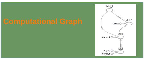
计算图的本质
一个计算图是由一系列 TensorFlow 操作组成的节点图。让我们构建一个简单的计算图。每个节点接受零个或多个张量作为输入,并产生一个张量作为输出。常量节点不接受任何输入。
请注意,仅仅打印节点本身并不会输出数值。我们只是定义了一个计算图,但还没有进行任何数值计算!
Pythonc1 = tf.constant([3.4, 9.1, -1.2, 9], dtype=tf.float64) c2 = tf.constant([3.4, 9.1, -1.2, 9], dtype=tf.float64) x = tf.multiply(c1, c1) y = tf.multiply(c1, c2) final_node = tf.add(x, y) print(c1) print(x) print(final_node)Output:
Tensor("Const_6:0", shape=(4,), dtype=float64) Tensor("Mul_6:0", shape=(4,), dtype=float64) Tensor("Add_3:0", shape=(4,), dtype=float64)要评估这些节点,我们必须在会话中运行计算图。会话封装了 TensorFlow 运行时的控制和状态。以下代码创建一个
Session对象,然后调用其run方法来运行计算图的足够部分以评估final_node。首先,我们创建一个会话对象:
Pythonsession = tf.Session()现在,我们可以通过启动会话对象的
run方法来评估计算图:Pythonresult = session.run(final_node) print(result) print(type(result))Output:
[ 23.12 165.62 2.88 162. ] <class 'numpy.ndarray'>当然,当我们完成时,我们需要关闭会话:
Pythonsession.close()然而,通常使用
with语句是更好的做法,正如我们在入门示例中所示,因为它可以确保会话在代码块结束时自动关闭,避免资源泄露。
与 NumPy 的相似性
我们将使用 NumPy 重写以下 TensorFlow 程序,以展示它们在操作上的相似之处。
TensorFlow 版本:
Pythonimport tensorflow as tf session = tf.Session() x = tf.range(12) # 创建一个从0到11的张量 print(session.run(x)) # 运行并打印张量 x 的值 x2 = tf.reshape(tensor=x, # 将 x 重新塑形为 3x4 的矩阵 shape=(3, 4)) x2 = tf.reduce_sum(x2, reduction_indices=[0]) # 对矩阵按列求和 (reduction_indices=[0] 表示对第0维求和) res = session.run(x2) # 运行并打印 x2 的值 print(res) x3 = tf.eye(5, 5) # 创建一个 5x5 的单位矩阵 res = session.run(x3) # 运行并打印 x3 的值 print(res)Output:
[ 0 1 2 3 4 5 6 7 8 9 10 11] [12 15 18 21] [[ 1. 0. 0. 0. 0.] [ 0. 1. 0. 0. 0.] [ 0. 0. 1. 0. 0.] [ 0. 0. 0. 1. 0.] [ 0. 0. 0. 0. 1.]]NumPy 版本 (功能类似):
Pythonimport numpy as np x = np.arange(12) # 创建一个从0到11的 NumPy 数组 print(x) x2 = x.reshape((3, 4)) # 将 x 重新塑形为 3x4 的矩阵 res = x2.sum(axis=0) # 对矩阵按列求和 (axis=0 表示对第0轴求和) print(res) x3 = np.eye(5, 5) # 创建一个 5x5 的单位矩阵 print(x3)Output:
[ 0 1 2 3 4 5 6 7 8 9 10 11] [12 15 18 21] [[ 1. 0. 0. 0. 0.] [ 0. 1. 0. 0. 0.] [ 0. 0. 1. 0. 0.] [ 0. 0. 0. 1. 0.] [ 0. 0. 0. 0. 1.]]
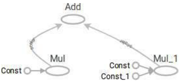
TensorBoard
TensorFlow 提供了借助名为 TensorBoard 的可视化工具来调试和优化程序的功能。
-
TensorFlow 在执行过程中会创建必要的数据。
-
这些数据存储在跟踪文件 (trace files) 中。
-
TensorBoard 可以通过浏览器访问
http://localhost:6006/来查看。
我们可以运行以下示例程序,它将创建一个名为 "output" 的目录。然后,我们可以运行
tensorboard --logdir output命令,它将启动一个 Web 服务器,并显示类似TensorBoard 0.1.8 at http://marvin:6006 (Press CTRL+C to quit)的信息。Pythonimport tensorflow as tf p = tf.constant(0.034) c = tf.constant(1000.0) x = tf.add(c, tf.multiply(p, c)) # x = c + p*c x = tf.add(x, tf.multiply(p, x)) # x = x + p*x with tf.Session() as sess: # 创建 FileWriter 对象,将计算图写入 "output" 目录 writer = tf.summary.FileWriter("output", sess.graph) print(sess.run(x)) # 运行并打印 x 的值 writer.close() # 关闭 FileWriterOutput:
1069.16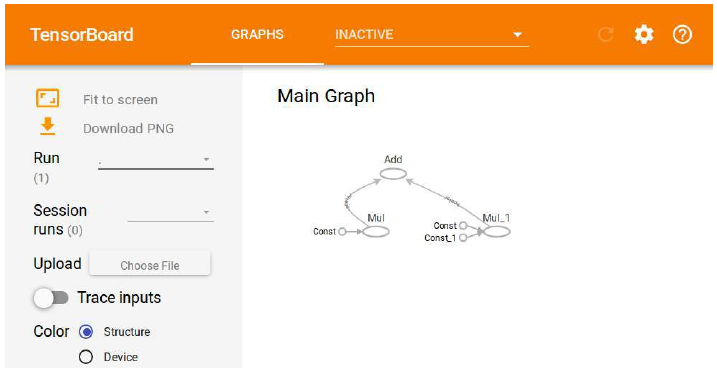
运行此代码后,您可以在 TensorBoard 中查看包含计算图的可视化结果。
占位符 (Placeholders)
计算图可以被参数化以接受外部输入,这些输入被称为占位符。占位符的值在会话运行图时提供。
Pythonimport tensorflow as tf # 定义两个占位符,它们的数据类型是 float32 c1 = tf.placeholder(tf.float32) c2 = tf.placeholder(tf.float32) # 定义使用占位符的计算操作 x = tf.multiply(c1, c1) y = tf.multiply(c1, c2) final_node = tf.add(x, y) with tf.Session() as sess: # 使用 .eval() 方法运行 final_node,并通过字典提供 c1 和 c2 的值 result = final_node.eval({c1: 3.8, c2: 47.11}) print(result) # 占位符也可以接受数组作为输入 result = final_node.eval({c1: [3, 5], c2: [1, 3]}) print(result)Output:
193.458 [ 12. 40.]另一个使用 NumPy 数组作为占位符输入的例子:
Pythonimport tensorflow as tf import numpy as np v1 = np.array([3, 4, 5]) v2 = np.array([4, 1, 1]) # 定义占位符,并指定形状为 (3,),表示一维数组,长度为 3 c1 = tf.placeholder(tf.float32, shape=(3,)) c2 = tf.placeholder(tf.float32, shape=(3,)) x = tf.multiply(c1, c1) y = tf.multiply(c1, c2) final_node = tf.add(x, y) with tf.Session() as sess: # 传入 NumPy 数组作为占位符的值 result = final_node.eval({c1: v1, c2: v2}) print(result)Output:
[ 21. 20. 30.]
tf.placeholder函数说明placeholder( dtype, shape=None, name=None )这个函数用于插入一个张量的占位符,该张量将始终被馈送 (fed)。它返回一个
Tensor对象,可以用作馈送值的句柄,但不能直接评估。重要提示:如果直接评估此张量,它将产生错误。它的值必须通过
feed_dict可选参数提供给以下方法:-
Session.run() -
Tensor.eval() -
Operation.run()
参数 (Args):
-
dtype: 要馈送的张量中元素的类型。 -
shape: 要馈送的张量的形状(可选)。如果未指定形状,则可以馈送任何形状的张量。 -
name: 操作的名称(可选)。
变量 (Variables)
变量用于向计算图添加可训练的参数。它们通过类型和初始值构建。当你调用
tf.Variable时,变量并不会立即被初始化。要初始化 TensorFlow 图中的所有变量,我们必须调用tf.global_variables_initializer:Pythonimport tensorflow as tf W = tf.Variable([.5], dtype=tf.float32) # 定义权重 W,初始值为 0.5 b = tf.Variable([-1], dtype=tf.float32) # 定义偏置 b,初始值为 -1 x = tf.placeholder(tf.float32) # 定义输入 x 的占位符 model = W * x + b # 定义线性模型:W * x + b with tf.Session() as sess: init = tf.global_variables_initializer() # 获取初始化所有变量的操作 sess.run(init) # 运行初始化操作,实际初始化 W 和 b print(sess.run(model, {x: [1, 2, 3, 4]})) # 运行模型并传入 x 的值Output:
[-0.5 0. 0.5 1. ]
变量与占位符的区别 (Difference Between Variables and Placeholders)
tf.Variable和tf.placeholder的区别在于值被传入的时间。-
如果你使用
tf.Variable,你必须在声明时提供一个初始值。 -
使用
tf.placeholder,你不需要提供初始值。它的值可以在运行时通过Session.run()中的feed_dict参数指定。
占位符用于将外部数据馈送到 TensorFlow 计算中,即从图外部传入!
如果你正在训练一个学习算法,占位符用于馈入你的训练数据。这意味着训练数据不是计算图的一部分。占位符的行为类似于 Python 的
input语句。另一方面,TensorFlow 变量的行为或多或少像一个 Python 变量!示例:计算损失 (Loss)
Pythonimport tensorflow as tf W = tf.Variable([.5], dtype=tf.float32) b = tf.Variable([-1], dtype=tf.float32) x = tf.placeholder(tf.float32) # 输入特征的占位符 y = tf.placeholder(tf.float32) # 真实标签的占位符 model = W * x + b # 定义模型预测值 deltas = tf.square(model - y) # 计算预测值与真实值之间的平方差 (误差) loss = tf.reduce_sum(deltas) # 计算所有误差的平方和,作为总损失 with tf.Session() as sess: init = tf.global_variables_initializer() # 初始化所有变量 sess.run(init) # 运行初始化操作 # 运行损失计算,并传入 x 和 y 的具体值 print(sess.run(loss, {x: [1, 2, 3, 4], y: [1, 1, 1, 1]}))Output:
3.5
重新赋值给变量 (Reassigning Values to Variables)
TensorFlow 变量的值可以在会话中通过
tf.assign()操作重新赋值。Pythonimport tensorflow as tf W = tf.Variable([.5], dtype=tf.float32) b = tf.Variable([-1], dtype=tf.float32) x = tf.placeholder(tf.float32) y = tf.placeholder(tf.float32) model = W * x + b deltas = tf.square(model - y) loss = tf.reduce_sum(deltas) with tf.Session() as sess: init = tf.global_variables_initializer() sess.run(init) print(sess.run(loss, {x: [1, 2, 3, 4], y: [1, 1, 1, 1]})) W_a = tf.assign(W, [0.]) # 创建一个将 W 赋值为 0.0 的操作 b_a = tf.assign(b, [1.]) # 创建一个将 b 赋值为 1.0 的操作 sess.run( W_a ) # 运行 W 的赋值操作 sess.run( b_a) # 运行 b 的赋值操作 # sess.run( [W_a, b_a] ) # 或者也可以在一次 'run' 调用中同时运行多个操作 print(sess.run(loss, {x: [1, 2, 3, 4], y: [1, 1, 1, 1]})) # 再次计算损失Output:
3.5 0.0可以看到,在重新赋值
W和b后,模型的损失从3.5变为0.0,这说明新的W=0和b=1使模型0*x+1 = 1完美匹配了目标y=[1,1,1,1]。
使用梯度下降优化器 (GradientDescentOptimizer)
以下示例展示了如何使用
tf.train.GradientDescentOptimizer来训练模型,使其最小化损失函数。Pythonimport tensorflow as tf W = tf.Variable([.5], dtype=tf.float32) b = tf.Variable([-1], dtype=tf.float32) x = tf.placeholder(tf.float32) y = tf.placeholder(tf.float32) model = W * x + b deltas = tf.square(model - y) loss = tf.reduce_sum(deltas) # 定义梯度下降优化器,学习率为 0.01 optimizer = tf.train.GradientDescentOptimizer(0.01) # 定义训练步骤:最小化损失函数 train = optimizer.minimize(loss) with tf.Session() as sess: init = tf.global_variables_initializer() # 初始化所有变量 sess.run(init) # 运行初始化操作 # 循环训练 1000 次 for _ in range(1000): sess.run(train, # 运行训练步骤 {x: [1, 2, 3, 4], y: [1, 1, 1, 1]}) # 传入训练数据 # 创建 FileWriter 用于 TensorBoard 可视化 writer = tf.summary.FileWriter("optimizer", sess.graph) print(sess.run([W, b])) # 打印训练后的 W 和 b 的值 writer.close() # 关闭 FileWriterOutput:
[array([ 3.91378126e-06], dtype=float32), array([ 0.99998844], dtype=float32)]经过 1000 次训练迭代,
W的值非常接近 0,而b的值非常接近 1,这与手动重新赋值时的理想值相符,表明梯度下降优化器有效地学习了模型参数。
创建数据集 (Creating Data Sets)
我们将为梯度下降优化器创建一个更大的分类示例数据集。这里我们将生成两类数据点:“bad ones” 和 “good ones”,并将其保存到文件中。
Pythonimport numpy as np import matplotlib.pyplot as plt # 循环创建训练集和测试集 for quantity, suffix in [(1000, "train"), (200, "test")]: # 生成“坏点”:均值为 [-2, -2],协方差为 [[1, 0], [0, 1]] 的多元正态分布 samples = np.random.multivariate_normal([-2, -2], [[1, 0], [0, 1]], quantity) # 绘制“坏点” plt.plot(samples[:, 0], samples[:, 1], '.', label="bad ones " + suffix) # 给“坏点”添加标签 0 bad_ones = np.column_stack((np.zeros(quantity), samples)) # 生成“好点”:均值为 [1, 1],协方差为 [[1, 0.5], [0.5, 1]] 的多元正态分布 samples = np.random.multivariate_normal([1, 1], [[1, 0.5], [0.5, 1]], quantity) # 绘制“好点” plt.plot(samples[:, 0], samples[:, 1], '.', label="good ones " + suffix) # 给“好点”添加标签 1 good_ones = np.column_stack((np.ones(quantity), samples)) # 将“坏点”和“好点”堆叠起来,形成完整的数据集 sample = np.row_stack((bad_ones, good_ones)) # 将数据集保存到文本文件 np.savetxt("data/the_good_and_the_bad_ones_" + suffix + ".txt", sample, fmt="%1d %4.2f %4.2f") plt.legend() # 显示图例 plt.show() # 显示图表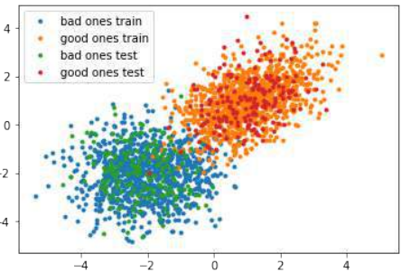
TensorFlow 模型的训练与评估
这是一个使用 TensorFlow 构建和训练一个简单分类模型的完整示例。模型将学习区分“好点”和“坏点”。
Pythonimport os # 抑制 TensorFlow 警告信息,设置日志级别为 ERROR os.environ['TF_CPP_MIN_LOG_LEVEL']='2' import numpy as np import tensorflow as tf from matplotlib import pyplot as plt # --- 超参数和配置 --- number_of_samples_per_training_step = 100 # 每个训练步骤(批次)的样本数 num_of_epochs = 1 # 训练的总轮数(此处为 1 轮) num_labels = 2 # 类别数量 (0 和 1) # --- 辅助函数定义 --- # 评估函数:使用模型对输入 X 进行预测 def evaluation_func(X): # predicted_class 是一个 TensorFlow 操作,需要通过 sess.run 或 .eval() 运行 return predicted_class.eval(feed_dict={x:X}) # 绘制决策边界函数 def plot_boundary(X, Y, pred_func): # 确定绘图画布的边界 mins = np.amin(X, 0) # 获取每列的最小值 mins = mins - 0.1*np.abs(mins) # 稍微扩展边界 maxs = np.amax(X, 0) # 获取每列的最大值 maxs = maxs + 0.1*maxs # 稍微扩展边界 # 创建网格点,用于在整个特征空间上评估模型 xs, ys = np.meshgrid(np.linspace(mins[0], maxs[0], 300), np.linspace(mins[1], maxs[1], 300)) # 使用密集的网格评估模型 # np.c_ 将扁平化的 xs 和 ys 组合成 (N, 2) 形状的数组,作为模型的输入 Z = pred_func(np.c_[xs.flatten(), ys.flatten()]) # 将模型输出的预测结果 Z 重新塑形回网格的形状 Z = Z.reshape(xs.shape) # 绘制等高线图和训练样本 # contourf 填充等高线区域,颜色对应不同的类别 plt.contourf(xs, ys, Z, colors=('c', 'g', 'y', 'b')) # 绘制真实数据点 Xn = X[Y[:,1]==1] # 提取标签为 1 的数据点 plt.plot(Xn[:, 0], Xn[:, 1], "bo", label="Good Ones") # 绘制蓝色圆点 Xn = X[Y[:,1]==0] # 提取标签为 0 的数据点 plt.plot(Xn[:, 0], Xn[:, 1], "go", label="Bad Ones") # 绘制绿色圆点 plt.legend() # 显示图例 plt.show() # 显示图表 # 加载数据函数 def get_data(fname): data = np.loadtxt(fname) # 从文件加载数据 labels = data[:, :1] # 提取第一列作为标签 (形状如 [[0.], [0.], [1.], ...]) # 将标签转换为独热编码 (one-hot encoding) 格式 labels_one_hot = (np.arange(num_labels) == labels).astype(np.float32) data = data[:, 1:].astype(np.float32) # 提取除了第一列的特征数据 return data, labels_one_hot # --- 数据加载 --- data_train = "data/the_good_and_the_bad_ones_train.txt" data_test = "data/the_good_and_the_bad_ones_test.txt" train_data, train_labels = get_data(data_train) # 加载训练数据 test_data, test_labels = get_data(data_test) # 加载测试数据 train_size, num_features = train_data.shape # 获取训练样本数和特征数 # --- TensorFlow 图的构建 --- # 定义输入特征的占位符 (x) 和真实标签的占位符 (y_) x = tf.placeholder("float", shape=[None, num_features]) # None 表示批次大小不固定 y_ = tf.placeholder("float", shape=[None, num_labels]) # 独热编码的标签 # 定义模型的权重 (Weights) 和偏置 (b) 变量,并初始化为零 Weights = tf.Variable(tf.zeros([num_features, num_labels])) b = tf.Variable(tf.zeros([num_labels])) # 定义模型的输出:使用 softmax 激活函数的逻辑回归模型 # tf.matmul(x, Weights) + b 实现线性变换 # tf.nn.softmax 将输出转换为概率分布 y = tf.nn.softmax(tf.matmul(x, Weights) + b) # --- 优化器和损失函数 --- # 定义交叉熵损失函数 cross_entropy = -tf.reduce_sum(y_*tf.log(y)) # 定义训练步骤:使用梯度下降优化器最小化交叉熵损失,学习率为 0.01 train_step = tf.train.GradientDescentOptimizer(0.01).minimize(cross_entropy) # 为测试数据创建常量节点,以便在评估时不传入 feed_dict test_data_node = tf.constant(test_data) # --- 评估指标 --- # 预测类别:tf.argmax(y, 1) 获取每个样本预测概率最大的类别索引 predicted_class = tf.argmax(y, 1) # 判断预测是否正确:tf.equal 比较预测类别和真实类别 correct_prediction = tf.equal(tf.argmax(y,1), tf.argmax(y_,1)) # 计算准确率:将布尔值转换为浮点数并求平均 accuracy = tf.reduce_mean(tf.cast(correct_prediction, "float")) # --- 会话运行和模型训练 --- with tf.Session() as sess: # 运行所有初始化器,准备可训练参数 (W 和 b) init = tf.global_variables_initializer() sess.run(init) # 迭代并训练模型 # 训练步数 = 总轮数 * (训练集大小 // 每个训练步的样本数) for step in range(num_of_epochs * train_size // number_of_samples_per_training_step): # 计算当前批次的起始偏移量 offset = (step * number_of_samples_per_training_step) % train_size # 获取当前批次的数据和标签 batch_data = train_data[offset:(offset + number_of_samples_per_training_step), :] batch_labels = train_labels[offset:(offset + number_of_samples_per_training_step)] # 将数据馈入模型并运行训练步骤 train_step.run(feed_dict={x: batch_data, y_: batch_labels}) # --- 训练结果输出 --- print('\n偏置向量 (Bias vector): ', sess.run(b)) print('权重矩阵 (Weight matrix):\n', sess.run(Weights)) print("\n应用于第一个数据集:") first = test_data[:1] # 获取测试数据的第一个样本 print(first) print("\nWx + b: ", sess.run(tf.matmul(first, Weights) + b)) # 打印线性模型的输出 # softmax 函数是一种广义的 logistic 函数,它将 K 维的任意实数向量 z “压缩”成一个 K 维的实数向量 σ(z), # 其值范围在 [0, 1] 之间且和为 1。 print("softmax(Wx + b): ", sess.run(tf.nn.softmax(tf.matmul(first, Weights) + b))) # 打印 softmax 输出 print("测试数据准确率 (Accuracy on test data): ", accuracy.eval(feed_dict={x: test_data, y_: test_labels})) print("训练数据准确率 (Accuracy on training data): ", accuracy.eval(feed_dict={x: train_data, y_: train_labels})) # --- 对新数据进行分类预测 --- print("\n对一些值进行分类:") print(evaluation_func([[-3, 7.3], [-1,8], [0, 0], [1, 0.0], [-1, 0]])) # 绘制决策边界 plot_boundary(test_data, test_labels, evaluation_func)Output:
偏置向量 (Bias vector): [-0.78089082 0.78089082] 权重矩阵 (Weight matrix): [[-0.80193734 0.8019374 ] [-0.831303 0.831303 ]] 应用于第一个数据集: [[-1.05999994 -1.55999994]] Wx + b: [[ 1.36599553 -1.36599553]] softmax(Wx + b): [[ 0.93888813 0.06111182]] 测试数据准确率 (Accuracy on test data): 0.97 训练数据准确率 (Accuracy on training data): 0.9725 对一些值进行分类: [1 1 1 1 0]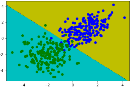
TensorFlow is an open-source software library for machine learning across a range of tasks. It is a symbolic
math library, and also used as a system for building and training neural networks to detect and decipher
patterns and correlations, analogous to human learning and reasoning. It is used for both research and
production at Google often replacing its closed-source predecessor, DistBelief. TensorFlow was developed by
the Google Brain team for internal Google use. It was released under the Apache 2.0 open source license on 9
November 2015.
TensorFlow provides a Python API as well as C++, Haskell, Java, Go and Rust APIs.
A tensor can be represented as a
multidimensional array of numbers. A
tensor has its rank and shape, rank is its
number of dimensions and shape is the
size of each dimension.
# a rank 0 tensor, i.e.
a scalar with shape ():
42
# a rank 1 tensor, i.e.
a vector with shape (3,):
[1, 2, 3]
# a rank 2 tensor, i.e. a matrix with shape (2, 3):
[[1, 2, 3], [3, 2, 1]]
# a rank 3 tensor with shape (2, 2, 2) :
[ [[3, 4], [1, 2]], [[3, 5], [8, 9]]]
#
Output:[[[3, 4], [1, 2]], [[3, 5], [8, 9]]]
All data of TensorFlow is represented as tensors. It is the sole data structure:
tf.float32, tf.float64, tf.int8, tf.int16, ..., tf.int64, tf.uint8, ...
437
STRUCTURE OF TENSORFLOW PROGRAMS
TensorFlow programs consist of two
discrete sections:
1.2.A graph is created in the
construction phase.
The computational graph is
run in the execution phase,
which is a session.
EXAMPLE
import tensorflow as tf
# Computational Graph:
c1 = tf.constant(0.034)
c2 = tf.constant(1000.0)
x = tf.multiply(c1, c1)
y = tf.multiply(c1, c2)
final_node = tf.add(x, y)
# Running the session:
with tf.Session() as sess:
result = sess.run(final_node)
print(result, type(result))
34.0012 <class 'numpy.float32'>
import tensorflow as tf
# Computational Graph:
c1 = tf.constant(0.034, dtype=tf.float64)
c2 = tf.constant(1000.0, dtype=tf.float64)
x = tf.multiply(c1, c1)
y = tf.multiply(c1, c2)
final_node = tf.add(x, y)
# Running the session:
438
with tf.Session() as sess:
result = sess.run(final_node)
print(result, type(result))
34.001156 <class 'numpy.float64'>
import tensorflow as tf
# Computational Graph:
c1 = tf.constant([3.4, 9.1, -1.2, 9], dtype=tf.float64)
c2 = tf.constant([3.4, 9.1, -1.2, 9], dtype=tf.float64)
x = tf.multiply(c1, c1)
y = tf.multiply(c1, c2)
final_node = tf.add(x, y)
# Running the session:
with tf.Session() as sess:
result = sess.run(final_node)
print(result, type(result))
[
23.12
165.62
2.88
162.
] <class 'numpy.ndarray'>
A computational graph is a series of TensorFlow operations arranged into a graph of nodes. Let's build a
simple computational graph. Each node takes zero or more tensors as inputs and produces a tensor as an
output. Constant nodes take no input.
Printing the nodes does not output a numerical value. We have defined a computational graph but no
numerical evaluation has taken place!
c1 = tf.constant([3.4, 9.1, -1.2, 9], dtype=tf.float64)
c2 = tf.constant([3.4, 9.1, -1.2, 9], dtype=tf.float64)
x = tf.multiply(c1, c1)
y = tf.multiply(c1, c2)
final_node = tf.add(x, y)

print(c1)
print(x)
print(final_node)
Tensor("Const_6:0", shape=(4,), dtype=float64)
Tensor("Mul_6:0", shape=(4,), dtype=float64)
Tensor("Add_3:0", shape=(4,), dtype=float64)
439
To evaluate the nodes, we have to run the computational graph within a session. A session encapsulates the
control and state of the TensorFlow runtime. The following code creates a Session object and then invokes its
run method to run enough of the computational graph to evaluate node1 and node2. By running the
computational graph in a session as follows. We have to create a session object:
session = tf.Session()
Now, we can evaluate the computational graph by starting the run method of the session object:
result = session.run(final_node)
print(result)
print(type(result))
[ 23.12 165.62   2.88 162.  ]
<class 'numpy.ndarray'>
Of course, we will have to close the session, when we are finished:
session.close()
It is usually a better idea to work with the with statement, as we did in the introductory examples!
SIMILARITY TO NUMPY
We will rewrite the following program with Numpy.
import tensorflow as tf
session = tf.Session()
x = tf.range(12)
print(session.run(x))
x2 = tf.reshape(tensor=x,
shape=(3, 4))
x2 = tf.reduce_sum(x2, reduction_indices=[0])
res = session.run(x2)
print(res)
x3 = tf.eye(5, 5)
res = session.run(x3)
print(res)
440
[ 0  1  2  3  4  5  6  7  8  9 10 11]
[12 15 18 21]
[[ 1.  0.  0.  0.  0.]
 [ 0.  1.  0.  0.  0.]
 [ 0.  0.  1.  0.  0.]
 [ 0.  0.  0.  1.  0.]
 [ 0.  0.  0.  0.  1.]]
Now a similar Numpy version:
import numpy as np
x = np.arange(12)
print(x)
x2 = x.reshape((3, 4))
res = x2.sum(axis=0)
print(res)
x3 = np.eye(5, 5)
print(x3)
[ 0  1  2  3  4  5  6  7  8  9 10 11]
[12 15 18 21]
[[ 1.  0.  0.  0.  0.]
 [ 0.  1.  0.  0.  0.]
 [ 0.  0.  1.  0.  0.]
 [ 0.  0.  0.  1.  0.]
 [ 0.  0.  0.  0.  1.]]
TENSORBOARD
••••TensorFlow provides functions to debug and optimize programs with the help of a visualization
tool called TensorBoard.
TensorFlow creates the necessary data during its execution.
The data are stored in trace files.
Tensorboard can be viewed from a browser using http://localhost:6006/
We can run the following example program, and it will create the directory "output" We can run now
tensorboard: tensorboard --logdir output
which will create a webserver: TensorBoard 0.1.8 at http://marvin:6006 (Press CTRL+C to quit)
import tensorflow as tf
p = tf.constant(0.034)
441
c = tf.constant(1000.0)
x = tf.add(c, tf.multiply(p, c))
x = tf.add(x, tf.multiply(p, x))
with tf.Session() as sess:
writer = tf.summary.FileWriter("output", sess.graph)
print(sess.run(x))
writer.close()
1069.16
The computational graph is included in the TensorBoard:
PLACEHOLDERS
A computational graph can be parameterized to accept external inputs, known as placeholders. The values for
placeholders are provided when the graph is run in a session.
442
import tensorflow as tf
c1 = tf.placeholder(tf.float32)
c2 = tf.placeholder(tf.float32)
x = tf.multiply(c1, c1)
y = tf.multiply(c1, c2)
final_node = tf.add(x, y)
with tf.Session() as sess:
result = final_node.eval( {c1: 3.8, c2: 47.11})
print(result)
result = final_node.eval( {c1: [3, 5], c2: [1, 3]})
print(result)
193.458
[ 12. 40.]
Another example:
import tensorflow as tf
import numpy as np
v1 = np.array([3, 4, 5])
v2 = np.array([4, 1, 1])
c1 = tf.placeholder(tf.float32, shape=(3,))
c2 = tf.placeholder(tf.float32, shape=(3,))
x = tf.multiply(c1, c1)
y = tf.multiply(c1, c2)
final_node = tf.add(x, y)
with tf.Session() as sess:
result = final_node.eval( {c1: v1, c2: v2})
print(result)
[ 21.
20.
30.]
placeholder( dtype, shape=None, name=None )
Inserts a placeholder for a tensor that will be always fed. It returns a Tensor that may be used as a handle for
feeding a value, but not evaluated directly.
Important: This tensor will produce an error if evaluated. Its value must be fed using the feed_dict optional
argument to
Session.run()
443
Tensor.eval()
Operation.run()
Args:
Parameter
Description
dtype:
The type of elements in the tensor to be fed.
shape:
The shape of the tensor to be fed (optional). If the shape is not specified, you can feed a tensor of any shape.
name:
A name for the operation (optional).
VARIABLES
Variables are used to add trainable parameters to a graph. They are constructed with a type and initial value.
Variables are not initialized when you call tf.Variable. To initialize the variables of a TensorFlow graph, we
have to call global_variables_initializer:
import tensorflow as tf
W = tf.Variable([.5], dtype=tf.float32)
b = tf.Variable([-1], dtype=tf.float32)
x = tf.placeholder(tf.float32)
model = W * x + b
with tf.Session() as sess:
init = tf.global_variables_initializer()
sess.run(init)
print(sess.run(model, {x: [1, 2, 3, 4]}))
[-0.5
0.
0.5
1. ]
DIFFERENCE BETWEEN VARIABLES AND PLACEHOLDERS
The difference between tf.Variable and tf.placeholder consists in the time when the values are passed. If you
use tf.Variable, you have to provide an initial value when you declare it. With tf.placeholder you don't have to
provide an initial value.
The value can be specified at run time with the feed_dict argument inside Session.run
A placeholder is used for feeding external data into a Tensorflow computation, i.e. from outside of the graph!
444
If you are training a learning algorithm, a placeholder is used for feeding in your training data. This means that
the training data is not part of the computational graph. The placeholder behaves similar to the Python "input"
statement. On the other hand a TensorFlow variable behaves more or less like a Python variable!
Example:
Calculating the loss:
import tensorflow as tf
W = tf.Variable([.5], dtype=tf.float32)
b = tf.Variable([-1], dtype=tf.float32)
x = tf.placeholder(tf.float32)
y = tf.placeholder(tf.float32)
model = W * x + b
deltas = tf.square(model - y)
loss = tf.reduce_sum(deltas)
with tf.Session() as sess:
init = tf.global_variables_initializer()
sess.run(init)
print(sess.run(loss, {x: [1, 2, 3, 4], y: [1, 1, 1, 1]}))
3.5
REASSIGNING VALUES TO VARIABLES
import tensorflow as tf
W = tf.Variable([.5], dtype=tf.float32)
b = tf.Variable([-1], dtype=tf.float32)
x = tf.placeholder(tf.float32)
y = tf.placeholder(tf.float32)
model = W * x + b
deltas = tf.square(model - y)
loss = tf.reduce_sum(deltas)
with tf.Session() as sess:
init = tf.global_variables_initializer()
sess.run(init)
print(sess.run(loss, {x: [1, 2, 3, 4], y: [1, 1, 1, 1]}))
445
W_a = tf.assign(W, [0.])
b_a = tf.assign(b, [1.])
sess.run( W_a )
sess.run( b_a)
# sess.run( [W_a, b_a] ) # alternatively in one 'run'
print(sess.run(loss, {x: [1, 2, 3, 4], y: [1, 1, 1, 1]}))
3.5
0.0
import tensorflow as tf
W = tf.Variable([.5], dtype=tf.float32)
b = tf.Variable([-1], dtype=tf.float32)
x = tf.placeholder(tf.float32)
y = tf.placeholder(tf.float32)
model = W * x + b
deltas = tf.square(model - y)
loss = tf.reduce_sum(deltas)
optimizer = tf.train.GradientDescentOptimizer(0.01)
train = optimizer.minimize(loss)
with tf.Session() as sess:
init = tf.global_variables_initializer()
sess.run(init)
for _ in range(1000):
sess.run(train,
{x: [1, 2, 3, 4], y: [1, 1, 1, 1]})
writer = tf.summary.FileWriter("optimizer", sess.graph)
print(sess.run([W, b]))
writer.close()
[array([ 3.91378126e-06], dtype=float32), array([ 0.99998844], dt
ype=float32)]
CREATING DATA SETS
We will create data sets for a larger example for the GradientDescentOptimizer.
import numpy as np
import matplotlib.pyplot as plt
446
for quantity, suffix in [(1000, "train"), (200, "test")]:
samples = np.random.multivariate_normal([-2, -2], [[1, 0],
[0, 1]], quantity)
plt.plot(samples[:, 0], samples[:, 1], '.', label="bad ones "
+ suffix)
bad_ones = np.column_stack((np.zeros(quantity), samples))
samples = np.random.multivariate_normal([1, 1], [[1, 0.5],
[0.5, 1]], quantity)
plt.plot(samples[:, 0], samples[:, 1], '.', label="good ones
" + suffix)
good_ones = np.column_stack((np.ones(quantity), samples))
sample = np.row_stack((bad_ones, good_ones))
np.savetxt("data/the_good_and_the_bad_ones_" + suffix + ".tx
t", sample, fmt="%1d %4.2f %4.2f")
plt.legend()
plt.show()
import os
os.environ['TF_CPP_MIN_LOG_LEVEL']='2'
import numpy as np
import tensorflow as tf
from matplotlib import pyplot as plt
number_of_samples_per_training_step = 100
num_of_epochs = 1
447
num_labels = 2 # should be automatically determined
defevaluation_func(X):
return predicted_class.eval(feed_dict={x:X})
def plot_boundary(X, Y, pred_func):
# determine canvas borders
mins = np.amin(X, 0)
# array with column minimums
mins = mins - 0.1*np.abs(mins)
maxs = np.amax(X, 0)
# array with column maximums
maxs = maxs + 0.1*maxs
xs, ys = np.meshgrid(np.linspace(mins[0], maxs[0], 300),
np.linspace(mins[1], maxs[1], 300))
# evaluate model using the dense grid
# c_ creates one array with "points" from meshgrid:
Z = pred_func(np.c_[xs.flatten(), ys.flatten()])
# Z is one-dimensional and will be reshaped into 300 x 300:
Z = Z.reshape(xs.shape)
# Plot the contour and training examples
plt.contourf(xs, ys, Z, colors=('c', 'g', 'y', 'b'))
Xn = X[Y[:,1]==1]
plt.plot(Xn[:, 0], Xn[:, 1], "bo")
Xn = X[Y[:,1]==0]
plt.plot(Xn[:, 0], Xn[:, 1], "go")
plt.show()
def get_data(fname):
data = np.loadtxt(fname)
labels = data[:, :1] # array([[ 0.], [ 0.], [ 1.], ...]])
labels_one_hot = (np.arange(num_labels) == labels).astype(np.f
loat32)
data = data[:, 1:].astype(np.float32)
return data, labels_one_hot
data_train = "data/the_good_and_the_bad_ones_train.txt"
data_test = "data/the_good_and_the_bad_ones_test.txt"
train_data, train_labels = get_data(data_train)
test_data, test_labels = get_data(data_test)
448
train_size, num_features = train_data.shape
x = tf.placeholder("float", shape=[None, num_features])
y_ = tf.placeholder("float", shape=[None, num_labels])
Weights = tf.Variable(tf.zeros([num_features, num_labels]))
b = tf.Variable(tf.zeros([num_labels]))
y = tf.nn.softmax(tf.matmul(x, Weights) + b)
# Optimization.
cross_entropy = -tf.reduce_sum(y_*tf.log)
train_step = tf.train.GradientDescentOptimizer(0.01).minimize(cros
s_entropy)
# For the test data, hold the entire dataset in one constant node.
test_data_node = tf.constant(test_data)
# Evaluation.
predicted_class = tf.argmax(y, 1)
correct_prediction = tf.equal(tf.argmax(y,1), tf.argmax(y_,1))
accuracy = tf.reduce_mean(tf.cast(correct_prediction, "float"))
with tf.Session() as sess:
# Run all the initializers to prepare the trainable parameter
s.
init = tf.global_variables_initializer()
sess.run(init)
# Iterate and train.
for step in range(num_of_epochs * train_size // number_of_samp
les_per_training_step):
offset = (step * number_of_samples_per_training_step) % tr
ain_size
# get a batch of data
batch_data = train_data[offsetoffset +
number_of_samples_per_trai
ning_step), :]
batch_labels = train_labels[offset
ples_per_training_step)]
449
s})
# feed data into the model
train_step.run(feed_dict={x: batch_data, y_: batch_label
print('\nBias vector: ', sess.run(b))
print('Weight matrix:\n', sess.run(Weights))
print("\nApplying model to first data set:")
first = test_data[:1]
print(first)
print("\nWx + b: ", sess.run(tf.matmul(first, Weights) + b))
# the softmax function, or normalized exponential function, i
s a generalization of the
# logistic function that "squashes" a K-dimensional vector z o
f arbitrary real values
# to a K-dimensional vector σ(z) of real values in the range
[0, 1] that add up to 1.
print("softmax(Wx + b): ", sess.run(tf.nn.softmax(tf.matmul(fi
rst, Weights) + b)))
print("Accuracy on test data: ", accuracy.eval(feed_dict={x: t
est_data, y_: test_labels}))
print("Accuracy on training data: ", accuracy.eval(feed_dic
t={x: train_data, y_: train_labels}))
# classify some values:
print(evaluation_func([[-3, 7.3], [-1,8], [0, 0], [1, 0.0],
[-1, 0]]))
plot_boundary(test_data, test_labels, evaluation_func)
450
Bias vector: [-0.78089082 0.78089082]
Weight matrix:
[[-0.80193734 0.8019374 ]
[-0.831303
0.831303 ]]
Applying model to first data set:
[[-1.05999994 -1.55999994]]
Wx + b: [[ 1.36599553 -1.36599553]]
softmax(Wx + b): [[ 0.93888813 0.06111182]]
Accuracy on test data: 0.97
Accuracy on training data: 0.9725
[1 1 1 1 0]
In [ ]:
In [ ]: -