Course: 2.13 中间值理论 | The Way To Learn

Section outline

Select section General

Collapse Expand
General

Collapse all Expand all
- Select activity 新闻通告
  
  新闻通告 Forum
Select section 中间值定理

Collapse Expand
中间值定理
This lesson introduces two theorems: The , and The Bounds on Zeros Theorem . A technical definition is given below, but what do these theorems really mean in 'ordinary language'?
::这个课程引入了两个理论: 和零点理论上的界圈。下面给出了一个技术定义,但这些理论在“普通语言”中究竟意味着什么?

Intermediate Value Theorem
::中间值定理

The intermediate value theorem offers one way to find roots of a continuous function. An informal definition of continuous is that a function is continuous over a certain interval if it has no breaks, jumps, asymptotes, or holes in that interval. Polynomial functions are continuous for all real numbers $\begin{aligned} x \end{aligned}$ . Rational functions are often not continuous over the set of real numbers because of asymptotes or holes in the graph, but for intervals without holes, rational functions are continuous.
::中间值定理为找到连续函数的根值提供了一种方法。对连续函数的非正式定义是,如果连续函数没有间断、跳跃、空洞或洞洞,则该连续函数会持续一段时间。对于所有真实数字来说,多数值函数都是连续的。由于图形中的空洞或空洞,理性函数通常不会连续超过一组真实数字,但是对于没有孔的间隔,理性函数是连续的。

If we know a function is continuous over some interval $\begin{aligned} [a, b] \end{aligned}$ , then we can use the intermediate value theorem :
::如果我们知道一个函数在某间距[a,b]内是连续的,那么我们可以使用中间值定理:

If $\begin{aligned} f (x) \end{aligned}$ is continuous on some interval $\begin{aligned} [a, b] \end{aligned}$ and $\begin{aligned} n \end{aligned}$ is between $\begin{aligned} f (a) \end{aligned}$ and $\begin{aligned} f (b) \end{aligned}$ , then there is some $\begin{aligned} c \in [a, b] \end{aligned}$ such that $\begin{aligned} f (c) = n \end{aligned}$ .
::如果f(x)在一定的间距[a、b]和n之间是连续的,则f(a)和f(b)之间是连续的,那么就有一些c[a、b],例如f(c)=n。

The following graphs highlight how the intermediate value theorem works. Consider the graph of the function $\begin{aligned} f (x) = \frac{1}{4} (x^{3} - \frac{5 x^{2}}{2} - 9 x) \end{aligned}$ below on the interval [-3, -1].
::下图显示中间值定理如何工作。请在 [ 3 - 1] 间距下方的函数 f( x) =14( x3 - 5x22 - 9x) 的图形。

$\begin{aligned} f (- 3) = - 5.625 \end{aligned}$ and $\begin{aligned} f (- 1) = 1.375 \end{aligned}$ . If we draw bounds on [-3, -1] and $\begin{aligned} [f (- 3), f (- 1)] \end{aligned}$ , then we see that for any $\begin{aligned} y - \end{aligned}$ value between $\begin{aligned} y = - 5.625 \end{aligned}$ and $\begin{aligned} y = 1.375 \end{aligned}$ , there must be an $\begin{aligned} x \end{aligned}$ value in [-3, -1] such that $\begin{aligned} f (x) = y \end{aligned}$ .
::f(-3)5.625和f(-1)=1.375。如果我们在[3-1)和[f(-3)、f(-1)]上划下界限,那么我们看到,对于y=5.625和y=1.375之间的任何y-值,[3-1]中必须有一个f(x)=y的x值。

So, for example, if we choose $\begin{aligned} c = - 2 \end{aligned}$ , we know that for some $\begin{aligned} x \in [- 3, - 1], f (x) = - 2, \end{aligned}$ even though solving this by hand would be a chore!
::例如,如果我们选择c2, 我们知道对于某些 x[-3,-1],f(x)2, 即使用手解决问题只是杂事!

The Bounds on Zeros Theorem is a corollary to the Intermediate Value Theorem:
::零点定理上的界圈是中间值定理的必然结果:

Bounds on Zeros Theorem
::零点定理上的弹道

If $\begin{aligned} f \end{aligned}$ is continuous on $\begin{aligned} [a, b] \end{aligned}$ and there is a sign change between $\begin{aligned} f (a) \end{aligned}$ and $\begin{aligned} f (b) \end{aligned}$ (that is, $\begin{aligned} f (a) \end{aligned}$ is positive and $\begin{aligned} f (b) \end{aligned}$ is negative, or vice versa), then there is a $\begin{aligned} c \in (a, b) \end{aligned}$ such that $\begin{aligned} f (c) = 0 \end{aligned}$ .
::如果f在[a,b]上是连续的,而且f(a)和f(b)(即f(a)为正数,f(b)为负数,或f(b)为负数,或反之亦然)之间有符号变化,那么就有一个f(c)=0的c(a),b)为f(c)=0。

The bounds on zeros theorem is a corollary to the intermediate value theorem because it is not fundamentally different from the general statement of the intermediate value theorem, just a special case where $\begin{aligned} n = 0 \end{aligned}$ .
::零定理上的界限是中间值定理的必然结果,因为它与中间值定理的一般说明没有根本的不同,只是n=0的一个特例。

Looking back at $\begin{aligned} f (x) = \frac{1}{4} (x^{3} - \frac{5 x^{2}}{2} - 9 x) \end{aligned}$ above, because $\begin{aligned} f (- 3) < 0 \end{aligned}$ and $\begin{aligned} f (- 1) > 0 \end{aligned}$ , we know that for some $\begin{aligned} x \in [- 3, - 1], f (x) \end{aligned}$ has a root. In fact, that root is at $\begin{aligned} x = - 2 \end{aligned}$ . and we can test that using synthetic division or by evaluating $\begin{aligned} f (- 2) \end{aligned}$ directly.
::回顾上文f(x)=14(x3-5x22-9x),因为f(-3) <0和f(-1)>0,我们知道,对于某些 x{{{[-3,-1],f(x)有根。事实上,根值为 x2,我们可以测试使用合成分解或直接评价f(-2)的方法。

Approximate Zeros of Polynomial Functions
::近乎零多元函数

In calculus you will learn several methods for numerically approximating the roots of functions. In this section we show one elementary numerical method for finding the zeros of a polynomial which takes advantage of the Intermediate Value Theorem.
::在微积分中,您将学习几种方法来从数字上接近函数根部。在本节中,我们展示了一种基本的数字方法,用以找到利用中间值理论的多元数值的零。

Given a continuous function $\begin{aligned} g (x) \end{aligned}$ ,
::给定连续函数 g( x) ,

Find two points such that $\begin{aligned} g (a) > 0 \end{aligned}$ and $\begin{aligned} g (b) < 0 \end{aligned}$ . Once you have found these two points, you can iteratively use the steps below to find the root of $\begin{aligned} g (x) \end{aligned}$ on the interval $\begin{aligned} [a, b] \end{aligned}$ . (Note, we will assume $\begin{aligned} a < b \end{aligned}$ , but the same algorithm works with minor adjustments if $\begin{aligned} b > a \end{aligned}$ )
::查找两个点, 如 g(a) > 0 和 g(b) < 0 。一旦您找到这两个点, 您可以反复使用下面的步骤在 [a, b] 间隔处找到 g(x) 根。 (注意, 我们会假设一个 < b , 但是如果 b> a , 同样的算法会稍作调整。

Evaluate $\begin{aligned} g (\frac{a + b}{2}) \end{aligned}$ .

If $\begin{aligned} g (\frac{a + b}{2}) = 0 \end{aligned}$ , then the root is $\begin{aligned} x = \frac{a + b}{2} \end{aligned}$ .
::如果 g( a+b2) =0, 那么根就是 x=a+b2 。

If $\begin{aligned} g (\frac{a + b}{2}) > 0 \end{aligned}$ , replace $\begin{aligned} a \end{aligned}$ with $\begin{aligned} \frac{a + b}{2} \end{aligned}$ . and repeat steps 1-2 using $\begin{aligned} [\frac{a + b}{2}, b] \end{aligned}$
::如果 g(a+b2) >0, 将 a 替换为 a+b2, 并使用 [a+b2, b] 重复步骤1-2

If $\begin{aligned} g (\frac{a + b}{2}) < 0 \end{aligned}$ , replace $\begin{aligned} b \end{aligned}$ with $\begin{aligned} \frac{a + b}{2} \end{aligned}$ . and repeat steps 1-2 using $\begin{aligned} [a, \frac{a + b}{2}] \end{aligned}$
::如果 g(a+b2) < 0, b 替换为 a+b2, 并使用 [a, a+b2] 重复步骤1-2

::评价 g(a+b2) g(a+b2) 。如果 g(a+b2) =0,则根为 x=a+b2=0; 如果 g(a+b2) >0, 根为 x=a+b2; 如果 g(a+b2) >0 , 以a+b2 取代a+b2; 重复步骤1-2 使用 [a+b2, b] 如果g(a+b2) <0, 则以b2 取代bb2 , 重复步骤1-2 使用[a, a+b2]

This algorithm will not usually find the exact root of $\begin{aligned} g (x) \end{aligned}$ , but it will allow you to find a reasonably small interval for the root. For example, you could repeat this process enough times so that you find an interval with $\begin{aligned} | a - b | < 0.01 \end{aligned}$ , and you will know the root of $\begin{aligned} g (x) \end{aligned}$ within a reasonably good approximation. The quality of the approximation you use (and the number of steps you use) will depend on why you are looking for the root. For most applications coming within 0.01 of the root is a reasonable approximation, but for some applications (such as building a bridge or launching a rocket) you need much more accuracy.
::此算法通常不会找到 g( x) 的准确根, 但允许您为 root 找到一个合理的小间隔。例如, 您可以重复此进程足够多的时间, 以便您在 {a- b\\\\\\\ 0.01 中找到一个间隔, 并且您可以在合理的好近似范围内知道 g( x) 的根。您使用的近似质量( 以及您使用的步数) 将取决于您为什么寻找根。对于 root 的 0.01 中的大多数应用程序来说, 是一个合理的近似值, 但对于某些应用程序( 如建桥或发射火箭) , 您需要更加精确。

An Interesting Corollary of the Intermediate Value Theorem
::《中间价值理论集》一首有趣的《中值理论集》

One surprising result of the Intermediate Value Theorem is that if you draw any great circle around the globe, then there must two antipodal points on that great circle that have exactly the same temperature.
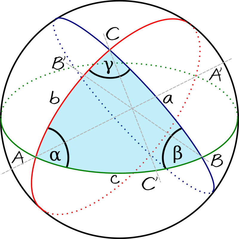
::中间值理论的一个令人惊讶的结果是,如果你在全球画出任何伟大的圆圈, 那么这个圆圈上必须有两个反聚变点, 温度完全一样。

Recall that a great circle is a path around a sphere that gives the shortest distance between any two points on the sphere. The equator is a great circle around the globe. Antipodal points are two points on opposite sides of the sphere. In the diagram below, $\begin{aligned} B \end{aligned}$ and $\begin{aligned} B^{'} \end{aligned}$ are antipodal.
::回顾一个大圆环是一个环绕球体的路径, 它使球体上任何两个点之间的距离最短。赤道环绕全球的大圆圈。反波达尔点是球体对面的两个点。在下面的图表中, B 和 B 和 B 是反波达尔。

For an informal proof of this result, look at the image of a sphere with three great circles above. Suppose that the temperature at $\begin{aligned} B \end{aligned}$ is $\begin{aligned} 75^{\circ} \end{aligned}$ and the temperature $\begin{aligned} B^{'} \end{aligned}$ is $\begin{aligned} 50^{\circ} \end{aligned}$ . The difference between the temperature at $\begin{aligned} B \end{aligned}$ and at $\begin{aligned} B^{'} \end{aligned}$ is $\begin{aligned} 75 - 50 = 25 \end{aligned}$ . Now imagine rotating the segment $\begin{aligned} \bar{B B^{'}} \end{aligned}$ around the blue great circle. When the segment has rotated 180 degrees (i.e. when $\begin{aligned} B \end{aligned}$ has rotated to where $\begin{aligned} B^{'} \end{aligned}$ is), then the difference between the temperatures at these two points is $\begin{aligned} 50 - 75 = - 25 \end{aligned}$ . Since temperatures vary continuously, by the intermediate value theorem, there must be some point on that circle when the difference was 0, implying two antipodal points had the same temperature.
::对于这一结果的非正式证明,请查看一个球体上方三个大圆的图象。假设B的温度是75°, B的温度是50°。 B和B的温度差是75- 50=25。现在想象一下在蓝色大圆圈周围旋转BB的段段。当该段旋转了180度( 即B旋转到B的位置) 时, 这两个点的温度差是50- 75°25。由于温度持续变化, 按中间值定理计算, 当差值是0时, 圆圈上一定有一些点, 意味着两个反波尔点的温度相同。

Notice that this little demonstration does not tell us which two antipodal points had the same temperature, only that there must be two such points on any great circle.
::请注意,这个小小的演示并没有告诉我们两个抗波变点的温度相同,只是指出在任何大圆圈上必须有两个这样的点。

Examples
::实例

Example 1
::例1

Earlier, you were asked if you could write less formal definitions of the Intermediate Value Theorem and the Bounds on Zeros Theorem .
::更早之前,有人问过你,你是否可以在零点定理上写出较不正式的中值定理和界圈定义。

One possibility might be:
::一种可能性是:

The Intermediate Value Theorem simply states that if you know two points on a graph, and know that the graph includes all the points between them, then any point between them must be on the graph.
::中间值定理仅仅指出,如果您知道图表上的两点,并且知道图表包括了它们之间的所有点,那么它们之间的任何点都必须在图表上。

The Bounds on Zeros Theorem suggests that if a graph contains all of the points between a positive and a negative value, then a zero point between those two values is on the graph.
::零点理论上的界点表示,如果一个图表包含正值和负值之间的所有点,则这两个值之间的零点在图形上。

Example 2
::例2

Show that $\begin{aligned} f (x) = - 3 x^{3} + 5 x \end{aligned}$ has at least one root in the interval [1, 2].
::显示 f( x)\\\\\\\\\\\\\\\\\\\\\\\\\\\\\\\\\\\\\\\\\\\\\\\\\\\\\\\\\\\\\\\\\\\\\\\\\\\\\\\\\\\\\\\\\\\\\\\\\\\\\\\\\\\\\\\\\\\\\\\\\\\\\\\\\\\\\\\\\\\\\\\\\\\\\\\\\\\\\\\\\\\\\\\\\\\\\\\\\\\\\\\\\\\\\\\\\\\\\\\\\\\\\\\\\\\\\\\\\\\\\\\\\\\\\\\\\\\\\\\\\\\\\\\\\\\\\\\\\\\\\\\\\\\\\\\\\\\\\\\\\\\\\\\\\\\\\\\\\\\\\\\\\\\\\\\\\\\\\\\\\\\\\\\\\\\\\\\\\\\\\\\\\\\\\\\\\\\\\\\\\\\\\\\\\\\\\\\\\\\\\\\\\\\\\\\\\\\\\\\\\\\\\\\\\\\\\\\\\\\\\\\\\\\\\\\\\\\\\\\\\\\\\\\\\\\\\\\\\\\\\\\\\\\\\\\\\\\\\\\\\\\\\\\\\\\\\\\\\\\\\\\\

Since $\begin{aligned} f (x) \end{aligned}$ is a polynomial we know that it is continuous. $\begin{aligned} f (1) = 2 \end{aligned}$ and $\begin{aligned} f (2) = - 14 \end{aligned}$ . Let $\begin{aligned} n = 0 \in [- 14, 2] \end{aligned}$ . Applying the Intermediate Value Theorem, there must exist some point $\begin{aligned} c \in [1, 2] \end{aligned}$ such that $\begin{aligned} f (c) = 0 \end{aligned}$ . This proves that $\begin{aligned} f (x) \end{aligned}$ has a root in [1, 2].
::由于 f( x) 是多数值, 我们知道它是连续的。 f( 1) = 2 和 f(2) 14。 Let n= 0 [ 14, 2] 。应用中间值理论, 必须存在某种点 c[ 1, 2] , 这样f( c) = 0 。这证明 f( x) 在 [ 1, 2] 中有根。

Example 3
::例3

The table below shows several sample values of a polynomial $\begin{aligned} p (x) \end{aligned}$ .
::下表显示了多元 p(x) 的若干样本值。

$\begin{aligned} x & - 4 & - 2 & 0 & 1 & 4 & 6 & 8 & 10 & 15 & 18 \\ p (x) & 44.15 & 6.62 & - 4.12 & - 4.09 & 1.16 & 0 & - 8.74 & - 24.07 & - 49.89 & 3.41 \end{aligned}$

::-4-2014-68101518p(x)44.156.62-4.12-4.91.160-8.74-24.07-49.893.41

Based on the information in the table:
::根据表中的资料:

a. What is the minimum number of roots of $\begin{aligned} p (x) \end{aligned}$ ?
::a. p(x) 最小根数是多少?

b. What are bounds on the roots of $\begin{aligned} p (x) \end{aligned}$ that you identified in (a)?
::b. 贵国在(a)项中所指明的p(x)的根底界限是什么?

Since $\begin{aligned} p (x) \end{aligned}$ is a polynomial we already know that it is continuous. We can use the Intermediate Value Theorem to identify roots by looking at when $\begin{aligned} p (x) \end{aligned}$ changes from negative to positive, or from positive to negative.
::由于 p( x) 是多元的, 我们已经知道它是连续的。我们可以使用中间值理论来识别根。我们可以通过查看p( x) 从负向正或从正向负的变化来识别根。

a. There are four sign changes of $\begin{aligned} p (x) \end{aligned}$ in the table, so at minimum, $\begin{aligned} p (x) \end{aligned}$ has four roots.
::a. 表中p(x)有4个符号变化,因此,至少p(x)有4个根。

b. The roots are in the following intervals $\begin{aligned} x \in [- 2, 0], x \in [1, 4], x \in [15, 18], \end{aligned}$ and the table also tells us that one root is at $\begin{aligned} x = 6 \end{aligned}$ .
::b. 根在以下间隔xx[-2,0],x{[1,4],x{[15,18],该表还告诉我们,一个根在x=6。

Example 4
::例4

Show the first 5 iterations of finding the root of $\begin{aligned} h (x) = x^{2} - x - 1 \end{aligned}$ using the starting values $\begin{aligned} a = 0 \end{aligned}$ and $\begin{aligned} b = 2 \end{aligned}$ .
::使用起始值 a=0 和 b=2 显示前 5 个查找 h( x) = x2 - x- 1 根根的迭代。

First we verify that there is a root between $\begin{aligned} x = 0 \end{aligned}$ and $\begin{aligned} x = 2 \end{aligned}$ . $\begin{aligned} h (0) = - 1 \end{aligned}$ and $\begin{aligned} h (2) = 1 \end{aligned}$ so we know there is a root in the interval [0, 2]. Check $\begin{aligned} h (\frac{2 + 0}{2}) = h (1) = - 1 \end{aligned}$ . Since $\begin{aligned} - 1 < 0 \end{aligned}$ we know the root is between $\begin{aligned} x = 1 \end{aligned}$ and $\begin{aligned} x = 2 \end{aligned}$ , and we use the new interval [1, 2].
::首先,我们核查 x=0 和 x=2. h(0) @% 1 和 h(2)=1 之间有一个根, 所以我们知道在间隔 [0, 2] 中有一个根。 check h( 2+02)=h(1)\\\\ 1. 因为-1 < 0 我们知道根在 x=1 和 x=2 之间, 我们使用新的间隔 [1, 2] 。

Now we use the interval [1, 2]. $\begin{aligned} h (\frac{1 + 2}{2}) = h (1.5) = - 0.25 \end{aligned}$ . Since $\begin{aligned} - 0.25 < 0 \end{aligned}$ , we use the interval [1.5, 2].
::现在我们使用间距[1, 2]. h(1+22)=h(1.5) @ @%0.25。从-0.25<0开始,我们使用间距[1.5, 2]。

$\begin{aligned} h (\frac{1.5 + 2}{2}) = h (1.75) = 0.31 \end{aligned}$ . Since $\begin{aligned} 0.31 > 0 \end{aligned}$ , we know that the zero is in the interval [1.5, 1.75].
::h(1.5+22)=h(1.75)=0.31。自0.31>0以来,我们知道零是间隔[1.5、1.75]。

$\begin{aligned} h (\frac{1.5 + 1.75}{2}) = h (1.625) = 0.02 \end{aligned}$ . Since $\begin{aligned} 0.02 > 0 \end{aligned}$ , we know the root is between 1.5 and 1.625.
::h(1.5+1.752)=h(1.625)=0.02。由于0.02>0,我们知道根在1.5到1.625之间。

$\begin{aligned} h (\frac{1.5 + 1.625}{2}) = h (1.5620) = - 0.12 \end{aligned}$ . Since $\begin{aligned} - 0.12 < 0 \end{aligned}$ , we know the root is between 1.5620 and 1.625.
::h(1.5+1.6252)=h(1.5620)=0.12。从-0.12 < 0开始,我们知道根在1.5620到1.625之间。

This example shows that after five iterations we have narrowed the possible location of the root to within 0.06 units. Not bad!
::这个例子显示,经过五次重复,我们已经将根的可能位置缩小到0.06个单位之内。不错!

Example 5
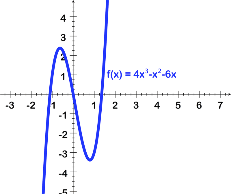
::例5

Use the image of the graph below to find the following:
::使用下图图的图像查找以下内容:

Degree of the polynomial
::多圆度

Number of real zeros and their approximate values using the graph
::使用图表的实际零数及其大致值

Number of imaginary zeros
::想象零数数

To identify the degree, recall that the degree of a polynomial is one number greater than the number of turns. The image shows turns at apx x = -.6 and apx x = .75, therefore this is a 3rd degree function.
::要识别度, 请提醒注意多角度的度比旋转数高一倍。图像显示以 apx x = - 6 和 apx x = . 75 旋转, 因此这是第 3 度函数。

The image shows the line crossing the x axis 3 times, at (apx) -1.15, at 0 and at (apx) 1.4.
::图像显示横跨 x 轴的线三次,在( px) - 1.15 处,0 和 (apx) 1.4 处。

Since this is a 3rd degree equation there are 3 possible zeros, and since there are 3 real zeros there are no imaginary ones.
::由于这是三级等式, 3个可能的零, 3个实际的零, 没有假想的零。

Example 6
::例6

Show that $\begin{aligned} f (x) = 8 x^{3} - 5 x^{2} - 7 x - 5 \end{aligned}$ has at least one root in the interval [1, 2].
::显示 f( x) = 8x3- 5x2- 7x- 5 在间隔[ 1, 2] 中至少有一个根。

Since $\begin{aligned} f (x) \end{aligned}$ is a polynomial we know that it is continuous. $\begin{aligned} f (1) = - 9 \end{aligned}$ and $\begin{aligned} f (2) = 25 \end{aligned}$ . Let $\begin{aligned} n = 0 \in [- 9, 25] \end{aligned}$ . Applying the Intermediate Value Theorem, there must exist some point $\begin{aligned} c \in [1, 2] \end{aligned}$ such that $\begin{aligned} f (c) = 0 \end{aligned}$ . This proves that $\begin{aligned} f (x) \end{aligned}$ has a root in [1, 2].
::由于 f( x) 是多数值, 我们知道它是连续的。 f(1)\\\\\\\\\\\\\\\\\\\\\\\\\\\\\\\\\\\\\\\\\\\\\\\\\\\\\\\\\\\\\\\\\\\\\\\\\\\\\\\\\\\\\\\\\\\\\\\\\\\\\\\\\\\\\\\\\\\\\\\\\\\\\\\\\\\\\\\\\\\\\\\\\\\\\\\\\\\\\\\\\\\\\\\\\\\\\\\\\\\\\\\\\\\\F(\\\\\\\\\\\\\\\\\\\\\\\\\\\\\\\\\\\\\\\\\\\\\\\\\\\\\\\\\\\\\\\\\\\\\\\\\\\\\\\\\\\\\\\\\\\\\\\\\\\\\\\\\\\\\\\\\\\\\\\\\\\\\\\\\\\\\\\\\\\\\\\\\\\\\\\\\\\\\\\\\\\\\\\\\\\\\\\\\\\\\\\\\\\\\\\\\\\\\\\\\\\\\\\\\\\\\\\\\\\\\\\\\\\\\\\\\\\\\\\\\\\\\\\\\\\\\\\\\\\\\\\\\\\\\\\\\\\\\\\\\\\\\\\\\\\\\\\\\\\\\\\

Note that since this is a 3rd degree polynomial, there are three zeros. Since there is only one real zero, the other two must be imaginary.
::请注意, 由于这是第三度多元度, 共有三点零。因为只有一个实际零, 另外两个必须是假想的。

Review
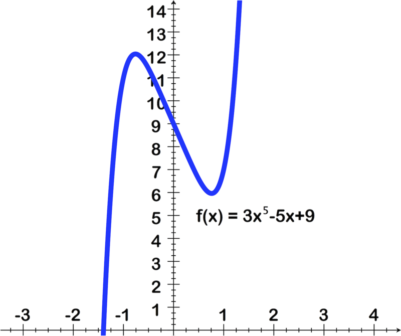
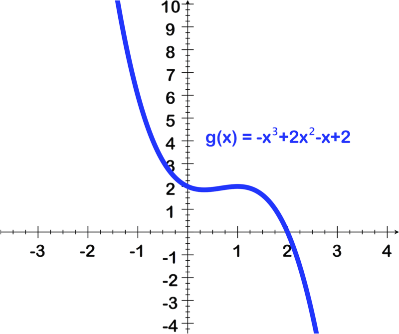
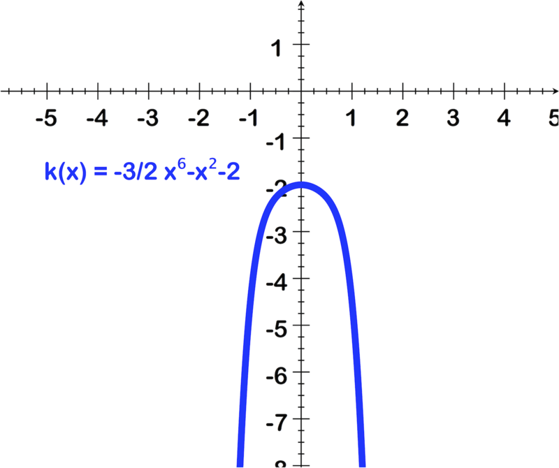
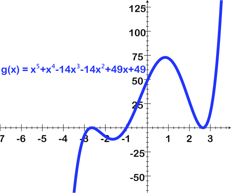
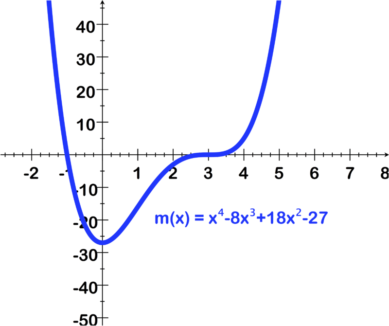
::回顾

For questions 1 - 6, use the image of the graph to find the following:
::对于问题1-6,请使用图中的图象来查找:

Leading coefficient and degree of the polynomial
::多民族体的主要系数和程度

Number of real zeros and their approximate values using the graph (Round your answer to the nearest hundredths)
::使用图形的实际零数及其近似值

Number of imaginary zeros
::想象零数数

For questions 7-12, use the intermediate value theorem to show the bounds on the zeros of each function. (Your bounds should be within the whole number)
::对于问题 7-12, 使用中间值定理来显示每个函数零的界限。 (你的界限应在整数之内)

$\begin{aligned} f (x) = 2 x^{3} - 3 x + 4 \end{aligned}$
:xx)=2x3-3x+4

$\begin{aligned} g (x) = - 5 x^{2} + 8 x + 12 \end{aligned}$
::g(x) =========================================================================================================================================================================================12===12

$\begin{aligned} h (x) = \frac{1}{2} x^{4} - x^{3} - 3 x^{2} + 1 \end{aligned}$
::h(x) = 12x4 - x3 - 3x2+1

$\begin{aligned} j (x) = - \frac{2}{x^{2} + 1} + \frac{1}{2} \end{aligned}$
::j(x) j( x) 2x2+1+12

$\begin{aligned} k (x) \end{aligned}$ is a polynomial and selected values of $\begin{aligned} k (x) \end{aligned}$ are given in the following table:
$\begin{aligned} x & - 3 & - 2 & - 1 & 0 & 1 & 2 & 3 \\ k (x) & - 23.5 & - 1 & 0.5 & - 1 & .5 & - 1 & - 23.5 \end{aligned}$

::k(x) 是多元值, 下表给出了 k(x) 的选定值 : x-3-2- 1 0 1 2 2 3k(x)- 23.5- 10.5-1.5-1- 23.5

Stephen argues the function $\begin{aligned} r (x) = \frac{4 x + 1}{x + 3.5} \end{aligned}$ has two zeros based on the following table and an application of the Bounds on Zeros Theorem. What is faulty about Stephen's reasoning?
$\begin{aligned} x & - 5 & - 4 & - 3 & - 2 & - 1 & 0 & 1 & 2 & 3 & 4 \\ r (x) & 12.67 & 30 & - 22 & - 4.67 & - 1.20 & 0.29 & 1.11 & 1.64 & 2.0 & 2.27 \end{aligned}$

::Stephen 辩称,函数 r(x) = 4x+1x+3.5 根据下表和零理论上的弹道应用有两个零。 Stephen 的推理有什么问题? x-5-4-3 - 2 - 1 0 1 2 3 4r (x) 12.67 30-22-4.67 - 1.200.291.111.64.2.02。

For questions 13-15, apply the numerical algorithm five times to find a bound on the zeros of the following functions given the indicated starting values.
::对于问题13-15, 5次使用数字算法, 以根据所示起始值, 在下列函数的零上找到约束值。

$\begin{aligned} k (x) = x^{4} - 3 x + 1 \end{aligned}$ on $\begin{aligned} [0, 1] \end{aligned}$
::[ 0, 1] 的 k(x) =x4- 3x+1

$\begin{aligned} b (x) = - 0.1 x^{5} + 3 x^{3} - 5 x^{2} \end{aligned}$ on $\begin{aligned} [1, 3] \end{aligned}$
:x) [1,3] b (x) 0.1x5+3x3-3-5x2

$\begin{aligned} c (x) = \frac{3 x^{2} - 2}{x^{4} + 2} \end{aligned}$ on $\begin{aligned} [0, 2] \end{aligned}$
:x)=3x2-2x4+2, [0, 2]

Review (Answers)
::回顾(答复)

Click to see the answer key or go to the Table of Contents and click on the Answer Key under the 'Other Versions' option.
::单击可查看答题键, 或转到目录中, 单击“ 其他版本” 选项下的答题键。

Section outline

General

中间值定理

Intermediate Value Theorem ::中间值定理

Bounds on Zeros Theorem ::零点定理上的弹道

Approximate Zeros of Polynomial Functions ::近乎零多元函数

An Interesting Corollary of the Intermediate Value Theorem ::《中间价值理论集》一首有趣的《中值理论集》

Examples ::实例

Example 1 ::例1

Example 2 ::例2

Example 3 ::例3

Example 4 ::例4

Example 5 ::例5

Example 6 ::例6

Review ::回顾

Review (Answers) ::回顾(答复)

Intermediate Value Theorem
::中间值定理

Bounds on Zeros Theorem
::零点定理上的弹道

Approximate Zeros of Polynomial Functions
::近乎零多元函数

An Interesting Corollary of the Intermediate Value Theorem
::《中间价值理论集》一首有趣的《中值理论集》

Examples
::实例

Example 1
::例1

Example 2
::例2

Example 3
::例3

Example 4
::例4

Example 5
::例5

Example 6
::例6

Review
::回顾

Review (Answers)
::回顾(答复)