4.11 历史和当前税务问题
章节大纲
-
Historical & Current Tax Issues
::历史和当前税务问题T he most current tax issues revolve around the idea that taxes are too high and that the tax laws should be much simpler. Some current concepts are to create value-added taxes, or a flat tax on individual income, or create more progressive tax brackets. Politicians and government officials revise taxes depending on the social and economic goals of their administrations, therefore tax laws can change from year to year and may either increase or decrease taxes on individuals, businesses or corporations.
::最新的税收问题围绕着税收过高和税法应该简单得多的理念。 目前的一些概念是创造增值税,或者个人收入的固定税,或者建立更累进的税括号。 政治家和政府官员根据行政部门的社会和经济目标修改税收,因此税法可以逐年改变,或者增加或者减少对个人、企业或公司的税收。Universal Generalizations
::普遍化-
The consequence of tax reform was to make the individual tax code more complex than ever.
::税制改革的结果是使个别税法比以往更加复杂。 -
Taxes influence the economy by affecting resource allocation, consumer behavior, and the nation’s productivity and growth.
::税收影响经济,影响资源分配、消费者行为和国家生产力和增长。 -
Taxes are the single most important way for the government to raise revenue.
::税收是政府增加收入的最重要的唯一方法。 -
Government economic policies at all levels influence levels of employment, output, and price levels.
::各级政府的经济政策影响就业、产出和价格水平。
Guiding Questions
::问 问 问 问 问 问 问 问 问 问 问 问 问 问 问 问 问 问 问 问 问 问 问 问 问 问 问 问 问 问 问 问 问 问 问 问 问 问 问 问 问 问 问 问 问 问 问 问 问 问 问 问 问 问 问 问 问 问 问 问 问 问 问 问 问 问 问 问 问 问 问 问 问 问 问 问 问 问 问 问 问 问 问 问 问 问 问 问 问 问 问 问 问 问 问 问 问 问-
How do the changing government policies of taxing affect the economy?
::不断变化的政府征税政策如何影响经济? -
What are the positive and negative aspects of taxation?
::税收的积极和消极方面是什么? -
How do taxes create a burden for the taxpayer?
::税收如何给纳税人造成负担?
The Kennedy Tax Cut of 1964
::1964年肯尼迪减税Now that we have some basic idea of how income taxes work, we turn to the Kennedy tax cut of 1964. We begin with some background information; we then develop the economic tools needed to analyze the effects of the tax policy on household consumption and therefore on real gross domestic product (real GDP).
::现在我们对所得税如何运作有了一些基本的认识,我们转向1964年肯尼迪减税。 我们首先从一些背景资料开始;然后我们开发必要的经济工具来分析税收政策对家庭消费,从而对实际国内生产总值(实际GDP)的影响。In his inaugural presidential address, President Kennedy famously said, “My fellow Americans, ask not what your country can do for you; ask what you can do for your country.” The Kennedy administration recruited top individuals in all fields (“the best and the brightest”) to come to Washington in this new spirit of commitment to public service.
::肯尼迪总统在总统就职演说中以“美国同胞们,不要问你们的国家能为你做什么;请问你们能为贵国做什么。” 肯尼迪政府招聘了所有领域的顶尖人士(“最优秀和最聪明的人”),本着这种致力于公共服务的新精神来到华盛顿。Every president has a group of economists that are known as the Council of Economic Advisors (CEA: ). They provide advice on economics and economic policy. The list of members and staff of the 1961 CEA reads today like a “who’s who” of economics. James Tobin and Robert Solow were prominent members of the economics team; both went on to win the Nobel Prize in Economics. The chairman of the CEA was Walter Heller, an economist known for a wide variety of contributions on the conduct of macroeconomic policy.
::每个总统都有一组被称为经济顾问委员会(CEA : ) 的经济学家。 他们提供经济学和经济政策方面的建议。 1961年CEA的成员和工作人员名单今天的解读就像经济学的“谁是谁 ” 。 詹姆斯·托宾和罗伯特·索洛是经济学团队的杰出成员,两人都赢得了诺贝尔经济学奖。 欧洲经济顾问委员会主席沃尔特·埃列尔(Walter Heller ) , 他是一位经济学家,对宏观经济政策的实施有着各种各样的贡献。The economists in the Kennedy administration observed that there had been three recessions in the two Eisenhower administrations (1952–1960): one from 1953 to 1954 after the Korean War, one from 1957 to 1958, and one in 1960. You can see these in Figure 1: "Real GDP in the 1950s". The CEA members and staff thought that more aggressive fiscal and monetary policies could be used to keep the economy more stable and prevent such recessions. Their goal of moderating fluctuations in the economy was based on the framework of the basic aggregate expenditure model, which had been developed in the aftermath of the Great Depression, modified by some developments in economic thinking from the 1940s and 1950s. Based on that analysis, they believed that fiscal and monetary policies could be used to control aggregate spending and hence real GDP.
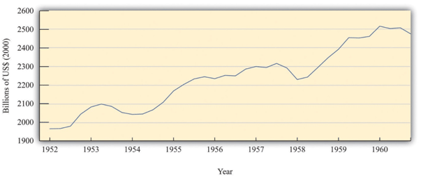
::肯尼迪政府的经济学家指出,在两个艾森豪威尔政府(1952-1960 ) , 经历了三次衰退(1952-1960 ) : 一次是朝鲜战争后从1953年到1954年的衰退,一次是1957年至1958年,另一次是1960年的衰退。 你可以在图1:“1950年代实际GDP ” ( Real GDP ) 中看到这一点。 中国经济研究中心的成员和工作人员认为,可以采用更激进的财政和货币政策来保持经济稳定并防止这样的衰退。 他们的经济波动调节目标基于在大萧条后发展的基本总开支模式框架,该模式由1940年代和1950年代经济思维的某些发展变化所修改。 基于这一分析,他们认为财政和货币政策可以用来控制总开支,从而控制实际GDP。Figure 1: Real GDP in the 1950s
::图1:1950年代实际国内生产总值Source: Bureau of Economic Analysis.
The chart shows real GDP in the United States between 1952 and 1960, measured in billions of year 2000 dollars.
This group of economists had, on one hand, a clearly defined goal of stabilizing the macroeconomy, and on the other hand, a set of policy instruments—economic variables such as taxes, government spending, and interest rates—that were under the control of policymakers. They also had a framework of analysis (the aggregate expenditure model) that explained how these instruments could be used to achieve their goals. Finally, they had a president who was willing to listen and take their advice. Never before had economists had such tools and wielded such influence.
::一方面,这组经济学家有一个稳定宏观经济的明确目标,另一方面,一套政策工具 — — 经济变量,如税收、政府支出和利率等 — — 由决策者控制。 他们还有一个分析框架(总开支模式 ) , 解释了如何利用这些工具实现其目标。 最后,他们有一个总统愿意倾听和听取他们的意见。 经济学家以前从未拥有过这样的工具,并运用过这样的影响力。The opportunity to test their ideas arose toward the middle of the Kennedy presidency. In the middle of 1962, it was apparent to the Kennedy administration economists that the economy was beginning to sputter. The growth rate of real GDP was 7.1 percent in 1959 but decreased to 2.5 percent and 2.3 percent in 1960 and 1961, respectively. Their response was to initiate a tax cut.
::测试他们想法的机会出现在肯尼迪总统任期的中间。 1962年年中,肯尼迪政府经济学家发现,经济开始崩溃。 1959年实际GDP增长率为7.1%,但1960年和1961年分别下降到2.5%和2.3%。 他们的反应是开始减税。As is usually the case when a major fiscal policy action is under consideration, there was a lengthy time lag between the initiation of the policy and its implementation. Even though the tax cut was proposed in 1962, President Kennedy never saw it put into effect. He was assassinated in November 1963; the tax cut for individual households and corporations was not enacted until early 1964. For households, tax withholding rates decreased from 18 percent to 14 percent, leading to an estimated tax reduction of about $6.7 billion. Taxes on corporations were also decreased; the reduction in taxes for 1964 was expected to be about $1.7 billion. By 1965, the economists expected that taxes would be lower by $11 billion. In 1965, nominal GDP was about $719 billion, so these changes were about 1.5 percent of nominal GDP.
::通常,在考虑采取重大财政政策行动时,从政策启动到实施之间有很长的时间间隔。尽管1962年提议减税,但肯尼迪总统从未看到减税生效。1963年11月,肯尼迪总统被暗杀;个人家庭和公司的减税直到1964年初才颁布。对于家庭来说,预扣税率从18%下降到14%,导致估计减税约67亿美元。公司税也有所减少;1964年减税约17亿美元。1965年,经济学家预计税收将降低110亿美元。1965年,名义GDP约为719亿美元,因此这些变化约为名义GDP的1.5%。For many observers of the macro-economy, this was a watershed event. The Economic Report of the President proclaimed 1965 the “Year of the Tax Cut.” In retrospect, these years were the heyday of Keynesian macroeconomics: for the first time, the government was using tax policy in an attempt to fine-tune the economy.
::对许多宏观经济观察者来说,这是一个分水岭事件。 《1965年总统经济报告》宣布1965年为“减税年 ” 。 回过头来看,这些年是凯恩斯宏观经济学的顶峰:政府首次利用税收政策试图调整经济。Figure 2: "Tax Policy during the Kennedy Administration" shows what happened to average and marginal tax rates. Marginal tax rates were very high at the time—much greater than in the present day. At high levels of income, more than 90 cents of every additional dollar had to be paid to the government in taxes. Consequently, average tax rates were also high: an individual with taxable income of $100,000 (a very high level of income back then) had to pay about two thirds of that amount to the government. The Kennedy tax cuts reduced these tax rates. Even after the tax cut, the marginal and average tax rates both increased with income. In other words, the tax system still redistributed income across households. But when we compare 1963 and 1964, we see that the marginal tax rate did not increase as rapidly under the new tax policy. Therefore, this channel of redistribution was weaker under the new tax policy.
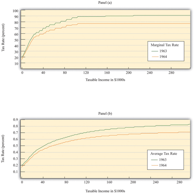
::图2:“肯尼迪政府时期的税收政策”显示了平均税率和边际税率的变化情况,边际税率当时非常高,比现在高得多,在高收入水平下,每增加一美元,就需要以税收形式向政府支付90多美分,因此,平均税率也很高:一个应纳税收入为10万美元(当时收入水平非常高)的人必须支付大约三分之二的税款给政府,肯尼迪减税减少了这些税率,即使减税之后,边际税率和平均税率都随着收入而增加。换句话说,税收制度仍然在家庭之间重新分配收入。但是,当我们比较1963年和1964年时,我们发现边际税率没有像新税收政策那样迅速增加。因此,在新的税收政策下,这种重新分配渠道比较弱。- Figure 2: Tax Policy During the Kennedy Administration
-
Source: Department of the Treasury, IRS 1987, “Tax Rates and Tables for Prior Years” Rev 9-87
The charts show the impact of the Kennedy tax cut. Part (a) highlights how the marginal tax rates for households changed from 1963 to 1964, and part (b) shows the impact on average tax rates. For their policy to be successful, Kennedy’s advisors had to ask and then answer a series of questions. How big a tax cut should they recommend? How long should it last? What would be the effect on government revenues? What would be the effect on real GDP and consumption? Economists working in government today confront exactly the same questions when contemplating changes in tax policy. Questions such as these epitomize economics and economists at work.
::图表显示了肯尼迪减税的影响。 (a)部分强调了1963年到1964年家庭边际税率的变化,(b)部分显示了对平均税率的影响。 肯尼迪顾问要成功,就必须询问并回答一系列问题。 他们建议减税要多大? 减税应该持续多久? 对政府收入有什么影响? 对实际GDP和消费会有什么影响? 在政府工作的经济学家在考虑改变税收政策时面临同样的问题。 这些问题包括经济学和经济学家在工作。Looking back at this experiment with almost half a century of hindsight, we can ask additional questions. How well did these policies work in terms of achieving their goal of economic stabilization? What actually happened to consumption and output? Was the tax policy successful?
::回顾这一近半个世纪的事后展望实验,我们可以提出更多的问题。 这些政策在实现经济稳定目标方面效果如何?消费和产出究竟发生了什么?税收政策是否成功?The Kennedy economists needed a quantitative model of economic behavior: a formalization of the links between their policy tools (tax rates) and the outcomes that they cared about, such as consumption and output. Using the aggregate expenditure model, they wanted to know how big a change in real GDP they could expect from a given change in the tax rate. To use the model to study income taxes, we need to add some theory about how spending responds to changes in taxes. Accordingly, we study the effects of income taxes on household consumption and then discuss how changes in consumption lead to changes in output.
::肯尼迪经济学家需要一个经济行为量化模型:将政策工具(税率)和他们关心的结果(如消费和产出)之间的联系正规化。 使用总开支模型,他们想知道他们从特定税率变化中预期实际GDP会有多大变化。 使用该模型研究所得税,我们需要增加一些关于支出如何应对税收变化的理论。 因此,我们研究所得税对家庭消费的影响,然后讨论消费变化如何导致产出变化。Although we are using a historical episode to help us understand the effect of taxes on the economy, this chapter is not intended as a lesson in economic history. Variations of this same model are still used today to analyze current economic policies. Indeed, in response to the economic crisis of 2008, many countries around the world cut taxes in an attempt to stimulate their economies. By studying the experience of the early 1960s, we gain insight into a critical part of macroeconomics: the linkage between consumption and output.
::尽管我们正在利用一个历史事件来帮助我们理解税收对经济的影响,但本章并不是经济史上的一个教训。 同样的模式在今天仍然被用来分析当前的经济政策。 事实上,为了应对2008年的经济危机,全世界许多国家都削减税收以刺激经济。 通过研究1960年代初的经验,我们深入了解了宏观经济的关键部分:消费与产出之间的联系。Having said that, economics has advanced significantly since the 1960s, and the state-of-the-art analysis for that time seems oversimplified today. Modern economists think that the policy advisers in the 1960s neglected some key aspects of the economy. Their insights were not wrong, but they were incomplete. Our understanding of the economy has evolved since Tobin, Solow, and Heller designed the nation’s tax policy.
::话虽如此,经济学自1960年代以来取得了显著进步,当时的最新分析今天似乎过于简单化了。 现代经济学家认为1960年代的政策顾问忽略了经济的某些关键方面。 他们的洞察力并不错误,但并不完全。 自托宾、索洛和埃列尔设计了国家税收政策以来,我们对经济的理解已经发生了演变。Household Consumption
::住户消费We begin by studying the relationship between consumption and income. We first develop some ideas about how households make consumption decisions, and, on the basis of those ideas, we make some predictions about what we expect to happen when there is a cut in taxes. We then examine the evidence from the Kennedy tax cut.
::我们首先研究消费与收入之间的关系。我们首先研究家庭如何决定消费。我们首先对家庭如何决定消费问题提出一些想法,并根据这些想法,我们对税收削减后预期会发生的事情作出一些预测。然后我们审查肯尼迪减税后的证据。Income, Consumption, and Saving
::收入、消费和储蓄Interested in studying, say, the market for ice cream? Examine how households choose between ice cream and other products that are close substitutes, (such as frozen yogurt), and between ice cream and other products that are complements, (such as hot fudge sauce). When studying microeconomics, however, we focus on choices for goods made at a particular point in time. In microeconomics, we study how a consumer allocates incomes across a wide variety of products.
::是否有兴趣研究冰淇淋市场? 研究家庭如何选择冰淇淋和其他贴近替代品的产品(如冰酸奶),以及冰淇淋和其他补充产品(如热果酱)之间的选择。 但是,在研究微观经济学时,我们专注于特定时间的商品选择。在微观经济学中,我们研究消费者如何将收入分配到各种各样的产品。Macroeconomics has a different emphasis. It emphasizes the choice between consumption and saving. Instead of thinking about the consumption of ice cream today versus frozen yogurt today, we study the choice between consumption today and consumption in the future. To highlight this decision, macroeconomists downplay the choices among different goods and services. Of course, in reality, households decide both how much to spend and how much to save, and what products to purchase. But it is convenient to treat these decisions separately.
::宏观经济有不同的强调。 它强调消费和储蓄之间的选择。 我们不考虑今天的冰淇淋消费和今天的冰酸奶,而是研究今天的消费和将来的消费之间的选择。为了突出这个决定,宏观经济学家低估了不同商品和服务之间的选择。 当然,在现实中,家庭决定支出多少和储蓄多少,以及购买什么产品。 但是,将这些决定分开处理是件容易的事。
The same basic ideas of household decision making apply in either case. Households distribute their income across goods to ensure that no redistribution of that spending would make them better off. This is true whether we are talking about ice cream and frozen yogurt, or about consumption and saving. Households allocate their income between consumption and savings in a way that makes them as well off as possible. They do not spend all their income this year because they want to save some for consumption in the future.
::家庭决策的基本理念在这两种情况下都适用。 家庭收入在货物之间分配,以确保支出的再分配不会使他们受益。 无论我们谈论的是冰淇淋和冰冻酸奶,还是消费和储蓄,这都是事实。 家庭收入在消费和储蓄之间分配的方式尽可能使他们受益。 今年,他们不把全部收入都花在商品之间,因为他们想将一些收入储蓄到未来的消费中。Suppose a household in the United States had taxable income of $20,000 in 2010. Some of this income goes to the payment of taxes to federal and state governments. (From our earlier discussion, the average federal tax rate is 13.25 percent.) The rest is either spent on goods and services or saved. The income that is spent on goods and services today is spread over the many products that a household buys. The income that is saved will likewise be used in the future to purchase different goods and services.
::假设美国家庭在2010年的应纳税收入为20,000美元,其中一些收入用于向联邦和州政府缴纳税款。 (根据我们先前的讨论,平均联邦税率为13.25%。 )其余收入要么用于商品和服务,要么用于储蓄。 如今,用于商品和服务的收入分散在家庭购买的许多产品上。 储蓄的收入也将在未来用于购买不同的商品和服务。Personal Income and Disposable Income
::个人收入和可支配收入The most basic measure of aggregate economic activity is real GDP, which is the total amount of final goods and services produced in our economy over a period of time, such as a year. The rules of national income accounting mean that real GDP measures three different things at once: the production or output of the economy, the spending in the economy; and the income generated in the economy. We use real GDP as our most general measure of income.
::衡量总体经济活动的最基本尺度是实际的国内生产总值,即我们经济在一年等一段时期内生产的最后货物和服务的总量,国民收入核算规则意味着实际国内生产总值同时衡量三种不同的情况:经济的生产或产出、经济支出以及经济产生的收入。 我们用实际国内生产总值作为我们收入的最一般衡量标准。We work in this chapter with two further concepts of income from the national accounts: personal income and disposable income. Some of the income generated in the economy is retained by firms to finance new investment, so it does not go to households. Personal income refers to that portion of GDP that finds its way directly into the hands of households. (At the level of an individual household, it corresponds closely to adjusted gross income on the tax form.) Disposable income is what remains after we subtract from personal income the taxes paid by households to the government and add to personal income the transfers (such as welfare payments) received by households from the government. For a household, disposable income measures its available resources after taxes have been paid and transfers received.
::在本章中,我们还有两个来自国民帐户的收入概念:个人收入和可支配收入;经济中产生的一些收入由公司保留,以资助新的投资,因此不用于家庭;个人收入是指直接掌握在家庭手中的国内生产总值的一部分。 (在个人家庭的水平上,它与税收表上调整后的毛收入十分吻合。 )可支配收入是我们从个人收入中扣除家庭向政府缴纳的税款之后的剩余收入,并在个人收入中加上家庭从政府收到的转款(例如福利付款),对于家庭而言,在纳税和收到转款之后,可支配收入衡量其可用资源。Consumption Smoothing
::消费平滑Our starting point for understanding consumption choices is the household budget constraint for a typical household. The household receives income from working and other sources and pays taxes to the government. The remainder is the household’s disposable income. The household budget constraint reminds us that, ultimately, you must either spend the income you receive or save it; there are no other choices. That is, disposable income = consumption + saving.
::我们理解消费选择的出发点是典型家庭的家庭预算限制。 家庭从工作和其他来源获得收入,并向政府纳税。 其余是家庭可支配收入。 家庭预算限制提醒我们,最终,你必须花掉或储蓄收入;没有其他选择。 也就是说,可支配收入=消费+储蓄。A theory of consumption is a theory of how households decide to divide their income between consumption and saving. Saving is a way to convert current income into future consumption. A theory of consumption is equivalently a theory of saving. A fundamental idea about household behavior is that people do not wish their consumption to vary a lot from month to month or year to year. This principle is so important that economists give it a special name: consumption smoothing. Households use saving and borrowing to smooth out fluctuations in their income and keep their consumption relatively smooth. People will tend to save when their income is high and will dissave when their income is low. (Dissave is the word economists use to mean either running down one’s existing wealth or borrowing against future earnings.)
::消费理论是家庭决定如何在消费和储蓄之间分配收入的理论。储蓄是将当前收入转换为未来消费的一种方法。消费理论相当于储蓄理论。关于家庭行为的基本理念是人们不希望他们的消费在逐月或逐年之间变化很大。 这一原则非常重要,经济学家给它一个特殊的名字:消费平稳。 家庭用储蓄和借款来缓解收入波动,保持相对的消费顺畅。 当他们的收入高时,人们倾向于储蓄,当他们的收入低时,他们就会分流。 (Dissave是经济学家用来指降低一个人现有的财富或以未来收入为代价的借款的词 ) 。Perfect consumption smoothing means that the household consumes exactly the same amount in each period of time (for example, a month or a year). If a construction worker earns $10,000 per month working from May to October but nothing for the rest of the year, we do not expect that he will spend $10,000 per month in the summer and then starve in the winter. It is much more likely that he will save half of his income in the summer and spend those savings in the winter so that he spends about $5,000 per month throughout the year.
::如果建筑工人从5月到10月每月挣10 000美元,但这一年的剩余时间却一无所获,我们并不期望他能在夏季每月花10 000美元,然后在冬季饿死,他更有可能在夏季省下一半的收入,在冬季花掉这些储蓄,以便他全年每月花大约5 000美元。The logic of consumption smoothing is the same as the argument for why households buy many different goods rather than one single good. Households typically take their income and spend it on a wide variety of products. Furthermore, when income increases, the household will spread this extra income across the spectrum of goods it consumes; not all of it is spent on one good. If you obtain more income, you do not spend all this extra income on ice cream, for example. You buy more of many different goods.
::消费平滑的逻辑与为什么家庭购买许多不同商品而不是单一商品的理由相同。 家庭通常把收入花在各种各样的产品上。 此外,当收入增加时,家庭将把额外收入分散到其消费的各种商品中,而不是全部花在一种商品上。如果你获得更多的收入,你就不会把这些额外收入全部花在冰淇淋上。例如,你买更多的不同商品。The Consumption Function
::消费职能One way to represent consumption smoothing is by means of a consumption function. This is an equation that relates current consumption to current disposable income. It allows us to go from an abstract idea about consumption behavior—consumption smoothing—to a specific formulation of consumption that we can use in a model of the aggregate economy.
::一种代表消费平滑的方法是通过消费功能来表示消费平滑。 这是一种将当前消费与当前可支配收入相联系的方程式。 它使我们能够从消费行为的抽象概念 — — 消费平滑 — — 转向我们可以在总经济模式中使用的具体消费配方。We suppose the consumption function can be represented by the following equation:
::我们认为消费功能可以用以下等式表示:- consumption = autonomous consumption + marginal propensity to consume × disposable income
- make three assumptions:
-
Autonomous consumption is positive
. Households consume something even if their income is zero. If the household has accumulated a lot of wealth in the past or if the household expects its future income to be larger, autonomous consumption will be larger. It captures both the past and the future.
::如果家庭在过去积累了大量财富,或者如果家庭预期其未来收入会增加,则自主消费将会增加,它会同时反映过去和未来。 -
We assume that the marginal propensity to consume is positive.
The marginal propensity to consume captures the present; it tells us how changes in current income lead to changes in current consumption. Consumption increases as current income increases; the larger the marginal propensity to consume, the more sensitive current spending is to current disposable income. By contrast, the smaller the marginal propensity to consume, the stronger is the consumption-smoothing effect.
::我们假设消费的边际倾向是积极的。 边际消费倾向抓住了现在;它告诉我们当前收入的变化如何导致当前消费的变化。 随着当前收入的增加,消费会增加;边际消费倾向越大,经常消费支出就越敏感。 相比之下,边际消费倾向越小,消费的边际倾向就越强,消费的平衡效应就越大。 -
We also assume that the marginal propensity to consume is less than one.
This says that not all additional income is consumed. When the household receives more income, it consumes some and saves some. The marginal propensity to save is the amount of additional income that is saved; it equals (1 – marginal propensity to consume).
::我们还假设,边际消费倾向低于一。 这说明并非所有的额外收入都得到消费。 当家庭收入增加时,它会消费一些,并节省一些。 边际储蓄倾向是储蓄的额外收入数量;它等于(1 ) — —消费的边际倾向 ) 。
Table 1 "Consumption, Income, and Saving" contains an example of a consumption function where autonomous consumption equals 10,000 and the marginal propensity to consume equals 0.8. If the household earns no income at all (disposable income = $0), it still spends $10,000 on consumption. In this case, savings equal −$10,000. This means the household is either drawing on existing wealth (accumulated savings from the past) or borrowing against income expected in the future. The marginal propensity to consume tells us how the household divides additional income between consumption and saving. In our example, the household spends 80 percent of any additional income and saves 20 percent.
::表1“消费、收入和储蓄”包含一个消费功能的例子,即自主消费等于10,000,消费的边际倾向等于0.8。如果家庭完全没有收入(可支配收入=0美元),它仍然在消费上花费10 000美元。在这种情况下,储蓄等于10,000美元。这意味着家庭要么利用现有财富(过去累积的储蓄),要么借入未来预期收入。消费边际倾向告诉我们家庭如何在消费和储蓄之间分配额外收入。例如,家庭花费任何额外收入的80%,节省20%。- Table 1: Consumption, Income, and Saving
Disposable Income ($)
::可支配收入(美元)Consumption ($)
::消费(美元)Saving ($)
:节省(美元))
0
10,000
−10,000
10,000
18,000
−8,000
20,000
26,000
−6,000
30,000
34,000
−4,000
40,000
42,000
−2,000
50,000
50,000
0
60,000
58,000
2,000
70,000
66,000
4,000
80,000
74,000
6,000
90,000
82,000
8,000
100,000
90,000
10,000
For example, when income is equal to $20,000, consumption can be calculated as follows:
::例如,当收入等于20 000美元时,消费可计算如下:consumption = $10,000 + 0.8 × $20,000
::消费=10 000美元+0.8美元×20 000美元= $10,000 + 0.8 × $20,000
= $26,000.
The household is still dissaving but now only by $6,000. Table 1 "Consumption, Income, and Saving" also shows that when income equals $50,000, consumption and income are equal, so savings are exactly zero. At income levels above $50,000, the household has positive savings.
::家庭仍然储蓄不足,但现在只有6 000美元。 表1“消费、收入和储蓄”也显示,当收入等于50 000美元时,消费和收入是相等的,因此储蓄是零。 在收入超过50 000美元时,家庭有正储蓄。Figure 3 "Consumption, Saving, and Income" shows the relationship between consumption and income graphically. We also graph the savings function in Figure 3 "Consumption, Saving, and Income". The savings function has a negative intercept because when income is zero, the household will dissave. The savings function has a positive slope because the marginal propensity to save is positive.
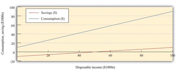
::图3“消费、储蓄和收入”用图形显示消费和收入之间的关系。我们也在图3“消费、储蓄和收入”中绘制储蓄功能图。储蓄功能有负截断功能,因为当收入为零时,家庭会分流。储蓄功能有一个正斜坡,因为储蓄的边际倾向是积极的。- Figure 3: Consumption, Saving, and Income
The graph shows the relationship between consumption and disposable income, where autonomous consumption is $10,000 and the marginal propensity to consume is 0.8. When disposable income is below $50,000, savings are negative, whereas at income levels above $50,000, savings are positive. As well as the marginal propensity to consume and the marginal propensity to save, we can examine the average propensity to consume, which measures how much income goes to consumption on average. It is calculated as follows:
::图表显示了消费和可支配收入之间的关系,其中自主消费为10 000美元,边际消费倾向为0.8。当可支配收入低于50 000美元时,储蓄为负值,而在收入水平超过50 000美元时,储蓄为正值。除了消费边际倾向和边际储蓄倾向外,我们可以检查平均消费倾向,衡量平均消费收入多少。计算如下:average propensity to consume = consumption /disposable income
::平均平均消费倾向 = 消费/可支配收入When disposable income increases, consumption increases but by a smaller amount. This means that when disposable income increases, people consume a smaller fraction of their income: the average propensity to consume decreases. In terms of mathematics, we are saying that, if we divide through the consumption function by disposable income, we get
::当可支配收入增加时,消费会增加,但增加量会小一些。 这意味着当可支配收入增加时,人们消费收入的一小部分是其收入的一小部分:消费平均倾向减少。 在数学方面,我们说,如果我们将消费功能除以可支配收入,我们就会得到Consumption = autonomous consumption + marginal propensity to consume
::消费=自主消费+边际消费倾向disposable income disposable income
::可支配收入可支配收入An increase in disposable income reduces the first term and the average propensity to consume. Meanwhile, the ratio of saving to disposable income is called the savings rate. For example,
::可支配收入的增加减少了第一个学期和消费的平均倾向。 与此同时,储蓄与可支配收入的比率被称为储蓄率。 例如,savings rate = savings disposable income.
::储蓄率=储蓄可支配收入。The savings rate and the average propensity to consume together sum to 1. In other words, a decline in the average propensity to consume equivalently means that households are saving a larger fraction of their income.
::储蓄率和平均消费倾向加起来等于1. 换句话说,平均消费倾向的下降意味着家庭正在节省收入的较大一部分。Because the consumption and savings relationships are two sides of the same coin, economists wishing to find the actual values of autonomous consumption and the marginal propensity to consume can examine data on consumption, savings, or both. If the data were perfect, we would get the same answer either way. For the United States, both consumption and savings data are readily available, but in some countries the data on savings may be of higher quality than the consumption data, in which case economists use savings data to understand consumption behavior.
::由于消费和储蓄关系是同一枚硬币的两面,希望找到自主消费和边际消费倾向的实际价值的经济学家可以检查消费、储蓄或两者的数据。 如果数据是完美的,无论哪种方法,我们都会得到同样的答案。 对于美国来说,消费和储蓄数据都是现成的,但在一些国家,储蓄数据的质量可能高于消费数据,在这种情况下,经济学家利用储蓄数据来理解消费行为。Some Warnings about the Consumption Function
::关于消费函数的一些警告The consumption function is useful because it captures two fundamental insights: households seek to smooth their consumption, but consumption nonetheless responds to current income. But the consumption function is really too simple.
::消费功能之所以有用,是因为它包含了两个基本见解:家庭寻求平滑消费,但消费仍然符合当前收入。 但消费功能实在太简单了。First, it ignor es the role of accumulated wealth. If you consider two households with the same level of current income but different amounts of accumulated wealth, the one with higher wealth will probably consume more. Second, the consumption function does not explicitly include the role of expectations. A household’s consumption reflects not only income today and the accumulation of income in the form of wealth but also anticipated income. So, for example, if a government announces that it will increase income tax rates in two years, we expect that households will respond immediately to smooth out the effects of these future taxes. The only way the consumption function allows us to capture wealth or expectations of future income is through autonomous consumption. This is fine as far as it goes, but it means that we are taking too many aspects of consumption as given, rather than explaining them with our theory.
::首先,它忽略了积累财富的作用。 如果你认为两个家庭目前的收入水平相同,但累积财富的数量却不同,那么财富较多的家庭可能会消费更多。 其次,消费功能并不明确包含期望的作用。 家庭消费功能不仅反映今天的收入,还反映财富形式的收入积累和预期收入。 因此,比如,如果政府宣布在两年内提高所得税率,我们预计家庭会立即作出反应以缓解这些未来税收的影响。 消费功能允许我们获取财富或对未来收入的期望的唯一方式就是自主消费。 就目前的情况来说,这很好,但这意味着我们采取了太多的消费方面,而不是用我们的理论来解释这些方面。Another complication is that changes in income today are often correlated with changes in income in the future. If your income increases today, is this an indication that your income will also be higher in the future? To see why this matters, consider two extreme examples. First, suppose that you receive a one-time inheritance of $10 million. What will you do with this income? According to the consumption smoothing argument, you will save some of this income to increase your consumption in the future. Roughly speaking, if you thought you had 10 years left to live, you might increase your consumption by about $1 million per year. In this case your marginal propensity to consume would be only 0.1.
::另一个复杂因素是,今天收入的变化往往与未来收入的变化相关。如果今天的收入增加,这是否表明你的收入在未来也会更高?为了了解这一点的原因,请考虑两个极端的例子。首先,假设你一次性获得1 000万美元的遗产。根据消费平滑的争论,你将节省部分收入以增加未来的消费。粗略地说,如果你认为你还有10年的寿命,你每年的消费可能会增加约100万美元。在这种情况下,你的边际消费倾向将只有0.1。Now suppose that instead of a $10 million windfall, you learn you will receive $1 million each year for the next 10 years. In this case, your income is already spread out over your lifetime. So, in this second case, you will again want to smooth your consumption. But since the increase in income will be maintained for your lifetime, you can increase your consumption by an amount equal to the increase in your income. Your marginal propensity to consume will be 1.0.
::现在假设不是1 000万美元的意外收入,而是1 000万美元的意外收入,你就会知道在未来10年中,你每年将得到100万美元。在这种情况下,你的收入已经分散在你的一生中。因此,在第二个情况下,你将再次想要平滑消费。但是,由于收入的增加将维持在你的一生中,你可以增加你的消费,其数额相当于收入的增加。你的边际消费倾向将是1.0。The difference between these two situations is that in the first case the income increase is temporary, and in the second it is permanent. The logic of consumption smoothing implies that the marginal propensity to consume is near 1 for permanent changes in income but much smaller for temporary changes in income.
::这两种情况之间的差别在于,在第一个情况中,收入增长是暂时性的,而在第二个情况中,收入增长是永久性的。 消费平滑的逻辑意味着边际消费倾向对于收入的长期变化来说接近于1,而对收入的临时变化来说则要小得多。The Effects of a Change in Income Taxes
::所得税变化的影响We can now figure out the effects of a cut in taxes on consumption and saving. A reduction in taxes will increase disposable income. From the consumption function, this results in an increase in consumption equal to the marginal propensity to consume times the increase in disposable income. The average propensity to consume decreases. To summarize, if taxes are cut in the economy, we expect to see the following:
::现在,我们可以找出削减消费和储蓄税的效果。 削减税收将增加可支配收入。 从消费功能来看,这导致消费增加,相当于边际消费倾向的消费与可支配收入增长的倍数。 平均消费倾向下降。 概括地说,如果在经济中削减税收,我们期望看到以下结果:-
An increase in disposable income
::可支配收入增加 -
An increase in consumption that is smaller than the increase in disposable income (that is, a marginal propensity to consume less than 1)
::消费的增加小于可支配收入的增加(即消费小于1的边际倾向) -
A decline in the average propensity to consume
::平均消费倾向下降
When natural scientists such as molecular biologists or particle physicists want to see how good their theories are, they conduct experiments. Economists and other social scientists have much less ability to carry out experiments—certainly at the level of the macroeconomy. The Kennedy tax cut, however, is like a “natural” experiment in that there was a major policy change that we can think of as a change in an exogenous variable. It is not, in truth, completely exogenous. We already explained that the tax cut was enacted in response to the poor performance of the economy. We are not badly misled by thinking of it as an exogenous event, however. We can therefore use it to see how well our theory performs. Specifically, we can look to see whether disposable income and consumption do behave as we have predicted.
::当分子生物学家或粒子物理学家等自然科学家想了解他们的理论有多好时,他们就会进行实验。经济学家和其他社会科学家进行实验的能力要小得多 — — 无疑是在宏观经济一级。然而,肯尼迪减税就像一个“自然”实验,因为我们可以认为这是一个重大的政策变化,它是一个外源变量的改变。事实上,它不是完全外源的。我们已经解释过,减税是针对经济表现不佳而实行的。我们并没有因为把它视为一种外源事件而受到误导。我们因此可以利用它来观察我们的理论表现如何。具体地说,我们可以看看可支配收入和消费是否像我们预想的那样表现良好。Empirical Evidence on Consumption
::消费经验证据Before we turn to those specific questions, let us examine some data on consumption.
::在我们讨论这些具体问题之前,让我们审查一些有关消费的数据。Figure 4 "Consumption and Income" shows the behavior of consumption and disposable income from 1962 to 2010. The measures of both income and consumption are in year 2005 dollars. This means that the nominal (money) levels of income and consumption for each of the years have been corrected for inflation, so that we can see how the real level of consumption relates to the real level of income.
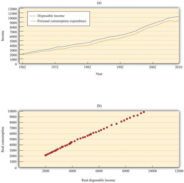
::图4“消费和收入”显示了1962年至2010年消费和可支配收入的行为。 收入和消费的衡量标准都是2005年美元。 这意味着每一年的名义(货币)收入和消费水平都因通货膨胀而得到纠正,这样我们就能看清实际消费水平与实际收入水平的关系。-
Figure 4: Consumption and Income
::图4:消费和收入
Source: Economic Report of the President (Washington, DC: GPO, 2011), table B-31, accessed September 20, 2011, http://www.gpoaccess.gov/eop/tables11.html.
The charts show consumption and personal disposable income (in billions of year 2005 dollars) from 1962 to 2010. Consumption and disposable income grew substantially over this time (a) and there is a close relationship between consumption and income (b).
::图表显示1962年至2010年的消费和个人可支配收入(2005年以10亿美元计),消费和可支配收入在此期间(a) 大幅增长,消费与收入(b) 关系密切。The first thing we see in Figure 4 "Consumption and Income" is that both consumption and disposable income grew substantially over the 1962–2010 period. This should come as no surprise. We know that the US economy grew over this period, so we would expect that disposable income and consumption would also grow. Figure 4 "Consumption and Income" reveals that, as a consequence, there is a close relationship between consumption and income, and consumption expenditures are, on average, about 91 percent of disposable income. Although Figure 4 "Consumption and Income" looks something like a consumption function, we should not take this relationship as strong evidence for our theory because it is primarily caused by the fact that both variables grew over time.
::在图4“消费和收入”中,我们看到的第一件事是消费和可支配收入在1962-2010年期间都大幅增长。 这并不令人惊讶。 我们知道美国经济在这一时期有所增长,因此我们预计可支配收入和消费也会增长。 图4“消费和收入”表明,消费和收入之间因此有着密切的关系,消费支出平均约为可支配收入的91%。 图4“消费和收入”看起来类似于消费功能,但我们不应该将这种关系视为我们理论的有力证据,因为它主要是两个变量随时间增长的结果。Consumption Response to the Kennedy Tax Cut
::对肯尼迪减税的消费反应Now we return to the Kennedy tax cut. How well does our model perform in predicting the effects of the tax changes on consumption? Superficially, this seems like an easy question. We can examine the changes in consumption and income that arose after the tax changes and see whether these changes are consistent with the model.
::现在,我们回到肯尼迪减税。 我们的模式在预测税收变化对消费的影响方面表现如何? 总体来说,这似乎是一个容易的问题。 我们可以研究税收变化后出现的消费和收入变化,看看这些变化是否与模式一致。There is a critical difference between our theory and reality, however. When we discussed the effects of a tax cut using our theory, we implicitly held everything else constant. We presumed that there was a change in taxes and no change in any other variable. For example, we assumed that government spending, investment spending, and net exports all did not change. In fact, other economic variables were changing at the same time that the new tax policy went into effect; these changes could also have affected consumption and disposable income. Looking at particular tax experiments is a messy business.
::然而,我们的理论和现实之间有着重大差异。 当我们用理论来讨论减税的效果时,我们暗含地保持了其他一切不变。 我们假设税收有变化,其他变量没有变化。 比如,我们假设政府支出、投资支出和净出口没有变化。 事实上,其他经济变量在新税收政策生效的同时也在变化;这些变化也可能影响消费和可支配收入。 具体税务实验是一个混乱的行业。Taxes were cut in February 1964, and (real) disposable income increased by $430 billion, a much larger increase than in previous time periods. Consumption expenditures increased considerably during this period. Table 2 "Consumption and Income in the 1960s (Seasonally Adjusted, Annual Rates)" summarizes the behavior of GDP, disposable income, consumption, and the average propensity to consume over the 1960–68 period. Remember that these are real variables, measured in year 2000 dollars. The average propensity to consume is calculated as consumption divided by disposable income, and the marginal propensity to consume is calculated as the change in consumption divided by the change in disposable income.
::1964年2月削减了税收,(实际)可支配收入增加了4300亿美元,比以往各时段的增长要大得多。 这一时期消费支出大幅增加。 表2“1960年代的消费和收入(季节性调整,年利率)”总结了1960-68年期间国内生产总值、可支配收入、消费和平均消费倾向的行为。 记住这些是真实变量,以2000年美元衡量。 消费的平均倾向是按可支配收入的消费除以可支配收入计算,消费的边际倾向是按可支配收入变化的消费变化计算的。Table 2: Consumption and Income in the 1960s (Seasonally Adjusted, Annual Rates)
::表2:1960年代的消费和收入(按季节调整的年率)Year
::年份 年份Real GDP ($)
::实际国内生产总值(美元)Disposable Income ($)
::可支配收入(美元)Consumption ($)
::消费(美元)APC
::APC 装甲运兵车MPC
::MPC MPC MPC MPC MPC MPC MPC MPC MPC MPC MPC MPC MPC MPC MPPC MPC MPC MPPC MPC MPC MPPC1960
2,501.8
1,759.7
1,597.4
0.91
—
1961
2,560.0
1,819.2
1,630.3
0.90
0.55
1962
2,715.2
1,908.2
1,711.1
0.90
0.91
1963
2,834.0
1,979.1
1,781.6
0.90
0.99
1964
2,998.6
2,122.8
1,888.4
0.89
0.74
1965
3,191.1
2,253.3
2,007.7
0.89
0.97
1966
3,399.1
2,371.9
2,121.8
0.89
0.96
1967
3,484.6
2,475.9
2,185.0
0.88
0.61
1968
3,652.7
2,588.0
2,310.5
0.89
1.11
-
     Source: Economic Report of the President (Washington, DC: GPO 2004), accessed September 20, 2011, .
     APC, average propensity to consume; MPC, marginal propensity to consume.
Disposable income increased as did consumption, in accordance with the predictions of our theory. As the theory predicts, the average propensity to consume decreased for most of this period. Likewise, in line with the theory, the marginal propensity to consume was less than 1 (in all years except 1968). Thus the evidence from this period is broadly consistent with the predictions that we made on the basis of our model.
::根据我们理论的预测,可支配收入与消费一样增加。正如理论预测的那样,平均消费倾向在这一期间大部分时间都有所下降。同样,根据理论,边际消费倾向低于1(1968年除外,1968年除外),因此这一时期的证据与我们根据模型所作的预测大致一致。Aggregate Income, Aggregate Consumption, and Aggregate Saving
::总收入、总消费和总储蓄The 1964 tax cut was not designed to influence consumption in isolation but rather to have an impact on the overall economy via its effect on consumption. So far, we have argued that a change in taxes leads to a change in disposable income and hence a change in consumption. Now we complete the story, noting that a change in consumption will itself affect the level of real GDP and hence have further effects on the level of disposable income.
::1964年减税的目的不是孤立地影响消费,而是通过其对消费的影响对整个经济产生影响。 到目前为止,我们一直认为税收的改变导致可支配收入的改变,从而导致消费的改变。 现在我们讲完这个故事,指出消费的改变本身将影响实际GDP水平,从而对可支配收入水平产生进一步的影响。In the case of the Kennedy tax cut of 1964, the economists advising the administration at that time had a fairly specific idea of how changes in consumption would affect the overall economy. They argued that the $10 billion tax cut would lead to an increase in GDP of about $20 billion each year. How did they create this estimate? To answer this question, we need to embed our theory of consumption in the aggregate expenditure model.
::就1964年肯尼迪减税而言,当时为政府提供咨询的经济学家对消费变化将如何影响整个经济有着相当具体的认识。 他们认为100亿美元的减税将导致GDP每年增加约200亿美元。 他们是如何得出这一估计的? 为了回答这个问题,我们需要把我们的消费理论纳入总支出模式。We motivated our consumption function by thinking about the behavior of an individual household. We now presume that our household is in some sense average, or representative of the entire economy, so the consumption relationship holds at an economy-wide level. Different households might actually have different consumption functions, but when we add them together, we still expect to find an aggregate relationship similar to the one we have described. The economists of the time used a framework that was closely based on the aggregate expenditure model. When prices are sticky, the level of GDP is determined in that model by the condition that planned spending and actual spending are equal. The model tells us that the level of real GDP depends on the level of autonomous spending and the multiplier,
::我们通过思考个体家庭的行为来激励我们的消费功能。我们现在假设我们的家庭在某种意义上是平均的,或代表整个经济,因此消费关系在全经济水平上维持着。不同的家庭可能实际上有不同的消费功能,但是当我们把它们加在一起时,我们仍然期望找到一个与我们所描述的相似的总关系。当时的经济学家使用一个密切基于总开支模式的框架。当价格粘糊时,以计划支出和实际支出相等的条件来确定该模式中的GDP水平。该模型告诉我们,实际GDP水平取决于自主支出水平和乘数,而实际GDP水平取决于自发支出水平和乘数。real GDP = multiplier × autonomous spending,
::实际国内生产总值=乘数x自主支出,where the multiplier is calculated as (11−marginal propensity to spend). Given the level of autonomous spending in the economy and given a value for the marginal propensity to spend, we can calculate the equilibrium level of real GDP.
::如果乘数计算为(11—边际消费倾向 ) 。 考虑到经济的自主支出水平以及边际消费倾向的价值,我们可以计算实际GDP的平衡水平。The marginal propensity to spend is not the same thing as the marginal propensity to consume, although they are connected. The marginal propensity to spend tells us how much total spending changes when GDP changes. Total spending includes not only consumption but also investment, government purchases, and net exports, so if any of these are responsive to changes in GDP, then the marginal propensity to spend is affected. Likewise, autonomous spending is not the same as autonomous consumption. Autonomous spending is the sum of autonomous consumption, autonomous investment, autonomous government purchases, and autonomous net exports. Finally, the marginal propensity to consume measures how consumption responds to changes in disposable income, not GDP.
::边际消费倾向与边际消费倾向不同,尽管它们相互关联。边际消费倾向告诉我们,当GDP变化时,总支出的变化有多大。 总支出不仅包括消费,还包括投资、政府购买和净出口,因此,如果其中任何一种对GDP变化作出反应,那么边际支出倾向就会受到影响。 同样,自主支出与自主消费不同。 自主支出是自主消费、自主投资、自主政府购买和自主净出口的和。 最后,消费的边际倾向是消费如何应对可支配收入变化,而不是GDP变化。In our analysis here, we continue to focus on consumption and suppose that the other components of spending—government spending, investment, and net exports—are exogenous. That is, these variables are all unaffected by changes in income and so are all included in autonomous spending. In addition, we presume that the amount that the government spends is not affected by the amount that it receives in tax revenue.
::在我们的分析中,我们继续关注消费问题,并假设政府支出、投资和净出口的其他组成部分是外来的。 也就是说,这些变数都不受收入变化的影响,因此都包括在自主支出中。 此外,我们假设政府支出的数额不受税收收入的影响。To find out the effects on the economy of a change in income taxes, we take the equation for real GDP and write it in terms of changes:
::为了了解所得税变化对经济的影响, 我们以实际GDP的等值来计算, 并用变化来写:change in real GDP = multiplier × change in autonomous spending.
::实际国内总产值变化=乘数x自主支出变化。This equation tells us we need two pieces of information to work out the effect of a tax change:
::这个方程式告诉我们我们需要两个信息 来判断税收变化的效果:-
The marginal propensity to spend because this allows us to calculate the multiplier
::支出的边际倾向 因为这让我们可以计算乘数 -
The effect of a tax change on autonomous spending
::税收变化对自主开支的影响
Let us think about the marginal propensity to spend first. We want to know the answer to the following question: if GDP changes by some amount (say, $100), what will happen to spending? There are three pieces to the answer.
::让我们想一想先花钱的边缘倾向。 我们想知道对以下问题的答案:如果GDP有一定数额的变化(比如100美元 ) , 支出会怎么样?答案有三个部分。-
A change in GDP leads to a change in personal income. Remember from the circular flow of income that GDP measures production, income, and expenditure in the economy. Firms receive income when they sell their products. Most of that income finds its way into the hands of households in the form of wage and salary payments or dividend payments. Firms hold onto some of the income that they generate to replace worn-out capital goods and finance new investments. In the early 1960s, personal income was about 78 percent of GDP. So if GDP increased by $100, we would expect personal income to increase by about $78.
::GDP的变化导致个人收入的改变。 记住,从收入循环流动中,GDP衡量生产、收入和经济支出。 公司在出售产品时获得收入。 大部分收入以工资和工资支付或股息支付的形式落入家庭手中。 公司持有其创造的某些收入以取代破旧的资本货物和为新投资提供资金。 1960年代初,个人收入约为GDP的78%。 因此,如果GDP增加100美元,我们预计个人收入将增加78美元。 -
A change in personal income leads, in turn, to a change in disposable income. As we explained at length, personal income is taxed, so disposable income is less than personal income. Since we are considering the effects of a change in taxes, we need an estimate of the marginal tax rate facing consumers. We know from Figure 27.3 that this varied across individuals, but researchers have estimated that for the economy as a whole, the marginal tax rate in 1964 was about 22 percent. Robert J. Barro and Chaipat Sasakahu provide estimates of the “average marginal tax rate.” Barro and Sasakahu, “Measuring the Average Marginal Tax Rate from the Individual Income Tax” (NBER Working Paper No. 1060 [Reprint No. r0487], June 1984), http://www.nber.org/papers/w1060. To put it another way, households would keep about 78 percent (= 100 percent – 22 percent) of their personal income. So if personal income increased by $78, disposable income would increase by about $61 (= 0.78 × $78). (It is a meaningless coincidence that these two numbers are both 78 percent.)
::个人收入的变化反过来又导致可支配收入的变化。 正如我们详细解释的那样,个人收入被征税,因此可支配收入比个人收入要少。由于我们考虑税收变化的影响,我们需要对消费者面临的边际税率进行估计。我们从图27.3中知道,这在个人之间有所不同,但研究人员估计,整个经济1964年的边际税率约为22%。Robert J. Barro和Chaipat Sasakahu提供了“平均边际税率”的估计数。 因此,如果个人收入增加78 % ( =100% - 22% ) , 那么,那么,如果个人收入增加78美元(=0.78×78美元 ) ,那么,从个人所得税中衡量平均边际税率(NBER工作文件第1060号[R0487号重刊 ,1984年6月 ) , http://www.nber.org/papers/w1060。 换句话说,家庭将保持其个人收入的78 % (=100% - 22% ) 。因此,如果个人收入增加68美元(=0.78美元) 。 -
Finally, a change in disposable income leads to a change in consumption. According to the 1964 Economic Report of the President, the CEA thought that the marginal propensity to consume was about 0.93. So if disposable income increased by $61, we would expect consumption to increase by about $57 (= 0.93 × $61).
::最后,可支配收入的变化导致了消费的变化。 根据1964年总统经济报告,中央经济审计局认为边际消费倾向约为0.93。 因此,如果可支配收入增加61美元,我们预计消费将增加57美元(=0.93×61美元 ) 。
Putting these three together, therefore, we see that an increase in GDP of $100 causes consumption to increase by $57. The marginal propensity to spend in this economy was equal to about 57 percent.
::因此,将这三个因素加在一起,我们看到,GDP增长100美元导致消费增加57美元。 在这一经济中支出的边际倾向相当于57%左右。Now let us think about the change in autonomous spending. We have said that taxes were cut by about $10 billion. We expect that most of this tax cut ended up in the hands of consumers. Based on the marginal propensity to consume of 0.93, we would, therefore, expect there to be an increase of about $9.3 billion in autonomous consumption,
::现在让我们想想自治支出的变化。 我们已经说过税收削减了约100亿美元。 我们预计大部分削减的税收最终都会落入消费者手中。 基于0.93的边际消费倾向,我们因此预计自主消费将增加93亿美元左右。change in autonomous spending = $9.3 billion.
::自主支出的变化=93亿美元。Putting these two results together, we find that our prediction for the change in GDP as a result of the tax cut is
::将这两个结果结合起来,我们发现,我们对由于减税而导致的国内生产总值变化的预测是:change in real GDP = multiplier × change in autonomous spending = 2.3 × $9.3 billion = $21.4 billion.
::实际国内总产值变化=乘数x自主支出变化=2.3×93亿美元=214亿美元。Our answer is not exactly equal to the $20 billion predicted by the CEA, but it is very close. As you might expect, the CEA was working with a more complicated model than the one we have explained here, and, as a result, they came up with a slightly smaller number for the multiplier.
::我们的答案并不完全等于中央能源局预测的200亿美元,但非常接近。 正如你可能预计的那样,中央能源局采用的模式比我们在此解释的复杂得多,因此,他们提出的乘数略小一些。A Word of Warning
::警告的一句话All our analysis so far has ignored the fact that, through the price adjustment equation, increased real GDP causes the price level to rise. This increase in prices serves to choke off some of the effects of the increase in spending. In effect, we have ignored the supply side of the economy. It is not that the Kennedy-Johnson administration economists were naïve about the supply side, but they thought the demand side movements were much more relevant for short-run policymaking purposes. More recent economic experience has convinced economists that we ignore the supply side of the economy at our peril. Modern macroeconomists would be careful to augment this story with a discussion of price adjustment.
::到目前为止,我们的所有分析都忽视了这样一个事实,即通过价格调整方程式,实际GDP的增长导致价格水平上升。价格的这一上升抑制了支出增长的某些影响。事实上,我们忽视了经济的供应方。 这并不是肯尼迪-约翰逊政府经济学家对供应方天真,而是他们认为需求方运动对于短期决策目的更为重要。 更近一些的经济经验让经济学家相信,我们忽视了经济的供应方,而我们却处于危险之中。 现代宏观经济学家会小心谨慎地通过讨论价格调整来补充这个故事。Tax Cuts and Private Saving
::减税和私人储蓄We have already conducted most of the analysis we need to examine the effects of tax cuts on saving. We know that a tax cut increases disposable income. Our theory of consumption smoothing tells us that households will respond by increasing consumption and savings. Specifically, we predict that a dollar’s worth of tax cuts will cause saving to increase by (1 − marginal propensity to consume). It is tempting to conclude that tax cuts, therefore, will lead both to higher consumption, increasing output now, and to higher saving, increasing output in the future. Such an argument is not right because it looks only at saving by households. We also need to look at the effect of the tax cut on the government surplus or deficit.
::我们已经进行了大部分必要的分析,以研究减税对储蓄的影响。 我们知道减税会增加可支配收入。 我们的消费平滑理论告诉我们,家庭会通过增加消费和储蓄来应对。 具体地说,我们预测,一美元的减税价值将导致储蓄增加(1 — — 边际消费倾向 ) 。 因此,人们很希望得出结论,减税将导致消费增加,现在的产量增加,将来的储蓄增加,产出增加。 这一论点是不正确的,因为它只着眼于家庭储蓄。 我们还需要研究减税对政府盈余或赤字的影响。Tax Cuts and National Saving
::减税和国家储蓄If the government is spending more than it receives in tax revenues, then it is running a deficit. Conversely, if it is spending less than it receives in tax revenues, it is running a surplus. National savings is the combined savings of the government and the private sector.
::如果政府的支出超过税收收入,那么它就会出现赤字。 相反,如果政府的支出低于税收收入,它就会出现盈余。 国民储蓄是政府和私营部门的储蓄。If the government is running a deficit, national savings = private savings − government deficit,
::如果政府出现赤字,国民储蓄=私人储蓄-政府赤字,If the government is running a surplus, national savings = private savings + government surplus.
::如果政府出现盈余,国民储蓄=私人储蓄+政府盈余。These are just two different ways of saying the same thing because, by definition, the government surplus equals minus the government deficit.
::这些只是两种不同的表达方式, 因为根据定义,政府盈余等于政府赤字减去政府赤字。What happens if the government cuts taxes? If there are no associated changes in government spending, then tax cuts translate dollar for dollar into the government budget. One million dollars worth of tax cuts will increase the deficit (or decrease the surplus) by exactly $1 million. So even though a tax cut of a dollar increases private savings by $(1 − marginal propensity to consume), it costs the government $1. The net effect (to begin with) is to reduce national savings by an amount equal to the marginal propensity to consume.
::如果政府削减税收? 如果政府支出没有相关变化,那么减税就会把美元换成政府预算。 价值100万美元的减税将把赤字(或顺差)增加100万美元。 因此,即使减税一美元使私人储蓄增加1美元 — — 即边际消费倾向,政府也要花1美元。 净效果(首先)是将国民储蓄减少相当于边际消费倾向的数额。If the tax cut succeeds in increasing income, there is additional savings resulting from the multiplier process. Still, we expect the overall effect is a decrease in national savings. For example, consider the Kennedy tax cut again. Taxes were cut by $10 billion. The resulting change in income was roughly $20 billion. With the marginal propensity to save equal to 0.07, the offsetting increase in private savings would have been about $1.4 billion. Evidently, the result was a large decrease in national savings.
::如果减税成功地增加了收入,那么乘数过程将产生额外的节余。 但我们预计总的效果是国民储蓄减少。 比如,再次考虑肯尼迪减税。 税收削减了100亿美元。 由此导致的收入变化约为200亿美元。 储蓄率勉强低于0.07,私人储蓄的抵消性增长将达到约14亿美元。 显然,结果是国民储蓄大幅下降。Here we see one of the biggest problems with tax cuts. They are attractive in the short run because they stimulate aggregate demand and increase output. They are also attractive politically, for obvious reasons. Unfortunately, they have the adverse long-run consequence of reducing national savings. When national savings decreases, the economy does not build up its capital stock so quickly, so future living standards are lower than they would otherwise be.
::我们在这里看到了减税的最大问题之一。 减税问题在短期内具有吸引力,因为它们刺激总需求和增加产出。 它们在政治上也具有吸引力,原因显而易见。 不幸的是,它们有着减少国民储蓄的长期不利后果。 当国民储蓄减少时,经济不会如此迅速地积累其资本存量,因此未来的生活水平比其他情况下要低。The Reagan Tax Cut
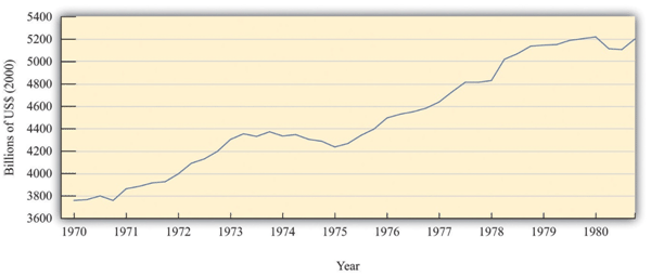
::里根减税When Ronald Reagan was elected US president in 1980, the US economy was not in very good shape. The 1970s had been a very difficult time for economies throughout the world. The oil-producing nations of the world, acting as a cartel, had increased oil prices substantially, and, as a result, energy costs had increased. These energy prices triggered a severe recession in the mid 1970s and a smaller recession in the late 1970s. Figure 5: "Real GDP in the 1970s" shows the US real gross domestic product (GDP) for this period. As well as recessions, the United States was suffering from inflation that was very high by historical standards: prices were increasing by more than 10 percent a year.
::当1980年罗纳德·里根当选美国总统时,美国经济的状态并不很好。 1970年代对全世界各经济体来说是一个非常困难的时期。 世界石油生产国作为卡特尔,大幅提高了石油价格,因此能源成本也随之上升。 这些能源价格引发了1970年代中期的严重衰退,1970年代后期的衰退规模较小。 图5 : “ 1970年代实际GDP ” 显示了这一时期的美国实际国内生产总值(GDP ) 。 以及衰退,美国也受到了以历史标准衡量非常高的通胀的影响:价格每年增长10%以上。Figure 5: Real GDP in the 1970s
::图5:1970年代实际国内生产总值Source: Bureau of Economic Analysis. The figure shows real GDP in the 1970s. There was a protracted recession in the mid-1970s and a smaller recession toward the end of the decade.
President Reagan and his economic advisors argued that high taxes were one of the causes of the relatively poor performance of the US economy. In particular, they claimed that taxes on income were deterring people from working as hard as they would otherwise. Unlike President Kennedy’s advisors, who had argued that income tax cuts would increase real GDP by stimulating aggregate expenditure, Reagan’s advisors said that tax cuts would increase potential output. Proponents of this economic view became known as supply siders because their focus was on the production of goods and services rather than the amount of spending on goods and services.
::里根总统及其经济顾问认为,高税收是美国经济表现相对差的原因之一。 特别是,他们声称所得税阻碍着人们像否则那样努力工作。 与肯尼迪总统的顾问不同,肯尼迪总统的顾问认为所得税削减会通过刺激总开支来增加实际GDP,但里根的顾问说减税会增加潜在产出。 这一经济观点的支持者被称作供应方,因为他们关注的焦点是商品和服务生产而不是商品和服务支出。After his inauguration, President Reagan pushed hard for changes in the tax code, and Congress enacted the Economic Recovery Tax Act (ERTA) in 1981. This law reduced tax rates substantially.
::里根总统就职后,大力要求修改税法,国会于1981年颁布了《经济复苏税法》,大幅降低了税率。The main mechanism that the supply-siders proposed was that lower income taxes would increase the incentive to work. To analyze this claim, we need to investigate how the decision to supply labor depends on income taxes. As with our analysis of consumption, we look at labor supply by thinking about the behavior of a single household. We then suppose that the household can be taken as representative of the entire economy.
::供方提出的主要机制是低所得税会增加工作激励。 为了分析这一主张,我们需要调查提供劳动力的决定如何取决于所得税。 与消费分析一样,我们通过思考一个家庭的行为来看待劳动力供给。 然后我们假设家庭可以被视为代表整个经济。Labor Supply
::劳动力供应Each individual faces a time constraint: there are only 24 hours in the day, which must be divided between working hours and leisure hours. An individual’s time budget constraint says that, on a daily basis, leisure hours + working hours = 24 hours.
::每个个人都面临时间限制:白天只有24小时,工作时间和休息时间必须分开。 个人预算限制规定,每天的休息时间+工作小时=24小时。The labor supply decision is equivalently the decision about how much leisure time to enjoy. This decision is based on the trade-off between enjoying leisure and working to purchase consumption goods. People like having leisure time, and they prefer more leisure to less. Leisure can be thought of as a “good,” just like chocolate or blue jeans or cans of Coca-Cola. People sacrifice leisure, working instead because the money they earn allows them to purchase goods and services.
::劳动供给决定与享受多少闲暇时间的决定是等同的。 该决定基于享受休闲和购买消费商品之间的权衡。 人们喜欢休闲时间,他们更喜欢闲暇而不是少闲暇。 闲暇可以被视为一种“好东西 ” , 就像巧克力、蓝色牛仔裤或可口可乐罐。 人们牺牲休闲,而工作是因为他们赚的钱可以购买商品和服务。To see this, we first rewrite the time budget constraint in money terms. The value of an hour of time is given by the nominal wage. Multiplying through the time budget constraint by the nominal wage gives us a budget constraint in dollars rather than hours:
::因此,我们首先用货币重写时间预算限制。一个小时的价值由名义工资来表示。 乘以时间预算限制,用名义工资来表示,我们的预算限制是以美元而不是以小时来表示:(leisure hours × nominal wage) + nominal wage income = 24 × nominal wage.
::+名义工资收入=24×名义工资。The second term on the left-hand side is “nominal wage income” since that is equal to the number of hours worked times the hourly wage.
::左侧的第二个术语是“名义工资收入”,因为这等于小时工资的工时数。Because wage income is used to buy consumption goods, we replace it by total nominal spending on consumption, which equals the price level times the number of consumption goods purchased:
::由于工资收入用于购买消费商品,我们用消费名义支出总额来取代,名义消费支出总额等于购买消费商品数量的价格水平的倍数:(leisure hours × nominal wage) + (price level × consumption) = 24 × nominal wage.
:This is the budget constraint faced by an individual choosing between consuming leisure and consumption. Think of it as follows: it is as if the individual first sells all her labor at the going wage, yielding the income on the right-hand side. With this income, she then “buys” leisure and consumption goods. The price of an hour of leisure is just the wage rate, and the price of a unit of consumption goods is the price level. Finally, if we divide this equation through by the price level, we see that it is the real wage (the wage divided by the price level) that appears in the budget constraint:
::这是个人在消费休闲和消费之间选择时面临的预算限制。 如下所述: 个人首先将所有劳动力按流动工资出售,在右侧产生收入。 有了这一收入,她就会“ 购买”闲暇和消费物品。 闲暇时间的价格只是工资率,而一个消费商品单位的价格是价格水平。 最后, 如果我们将这个等式除以价格水平,我们可以看到预算限制中出现的实际工资(工资除以价格水平 ) :(leisure hours × real wage) + consumption = 24 × real wage.
:It is the real wage, not the nominal wage, that matters for the labor supply decision.
::实际工资,而不是名义工资,是劳动力供应决定所必须的。Changes in the Real Wage
::实际工资的变化What happens if there is an increase in the real wage? There are two effects:
::如果实际工资增加,会发生什么情况?有两种影响:-
There is a substitution effect. An increase in the real wage means that leisure has become relatively more expensive. You have to give up more consumption goods to get an hour of leisure time. If leisure becomes more expensive, we would expect the household to “buy” fewer hours of leisure and more consumption goods—that is, to substitute from leisure to consumption. This effect predicts that the quantity of labor supplied will increase.
::有替代效应。 实际工资的增加意味着休闲变得相对昂贵。 您必须放弃更多的消费商品以获得一个小时的闲暇时间。 如果闲暇变得更加昂贵,我们将期望家庭“购买”更少的闲暇时间和更多的消费商品,也就是从闲暇到消费的替代。 这一效应预示着所供应的劳动力数量将会增加。 -
There is an income effect. An increase in the real wage makes the individual richer—remember that we can think of income as equaling 24 × the real wage. In response to higher income, we expect to see the household increase its consumption of goods and services and also increase its consumption of leisure. This effect predicts that the quantity of labor supplied will decrease.
::实际工资的增加使得个人富人想起,我们可以认为收入等于实际工资的24×。 为了应对收入的增加,我们预期家庭会增加商品和服务的消费,同时也会增加闲暇的消费。 这一影响预示所提供的劳动力数量将会减少。
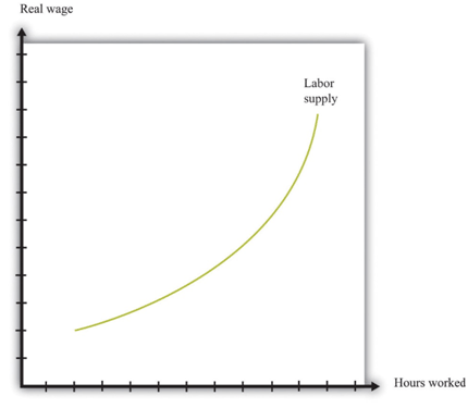
Putting these predictions together, we must conclude that we do not know what will happen to the quantity of labor supplied when the real wage increases. On the one hand, higher real wages make it attractive to work more since you can get more goods and services for each hour of time that you give up (the substitution effect). On the other hand, you can get the same amount of consumption goods with less effort, which makes it attractive to work less (the income effect). If the substitution effect is stronger, the labor supply curve has the standard shape: it slopes upward, as in Figure 6: "Labor Supply".
::把这些预测放在一起,我们必须得出这样的结论:当实际工资增加时,我们不知道提供劳动力的数量会发生什么。 一方面,较高的实际工资使工作更有吸引力,因为只要放弃(替代效应 ) , 每一小时你可以得到更多的商品和服务(替代效应 ) 。 另一方面,你可以以更少的劳动力获得同样数量的消费商品,这让工作更少(收入效应 ) 。 如果替代效应更强,则劳动力供应曲线具有标准形状:它向上倾斜,如图6中的数字 : “ 劳动供给 ” 。- Figure 6: Labor Supply
The response of the quantity of labor supplied to the real wage depends on both an income effect and a substitution effect. When the substitution effect is larger than the income effect, the supply curve has the “normal” upward-sloping shape.
::实际工资的劳动力数量反应取决于收入效应和替代效应。 当替代效应大于收入效应时,供应曲线具有“正常”向上倾斜的形状。In the end, the shape of the labor supply curve is an empirical question; we can answer it only by going to the data. And as you might be able to guess, it turns out to be a difficult question to answer, once we start dealing with the complexities of different kinds of labor. The view of most economists who have studied labor supply is that higher real wages do lead to a greater quantity of labor supplied, but the effect is not very strong. The income effect almost cancels out the substitution effect. This means that the labor supply curve slopes upward but is quite steep.
::最后,劳动力供给曲线的形状是一个经验性问题;我们只能通过使用数据来回答它。正如你可能能够猜想的那样,一旦我们开始处理不同类型劳动力的复杂性,这个问题就是一个难以回答的问题。 大多数研究过劳动力供给的经济学家都认为,更高的实际工资确实导致更多的劳动力供应,但效果并不很大。 收入效应几乎抵消了替代效应。 这意味着劳动力供给曲线向上倾斜,但相当陡峭。The Effect of the Reagan Tax Cuts on the Supply of Labor
::里根减税对劳动力供应的影响Suppose an individual knows the nominal wage but also knows that she is going to be taxed on any income that she earns at the going income tax rate. The wage rate that matters for her decision is the after-tax real wage. Her real disposable income is:
::假设个人知道名义工资,但也知道她将对其按流动所得税率赚取的任何收入征税。 对其决定至关重要的工资率是税后实际工资。 她的实际可支配收入是:disposable income = hours worked×(1−tax rate)×(nominal wage/price level)
::可支配收入=小时工作xx(1-税率)x(名义工资/价格水平)= hours worked×(1−tax rate)×real wage.
::=小时工作xx(1-税率)x实际工资。All our discussion of labor supply continues to hold in this case, except that we need to replace the real wage with the after-tax real wage since it is the after-tax wage that matters to the individual.
::我们关于劳动力供应的所有讨论在此案中依然有效,只是我们需要以税后实际工资取代实际工资,因为对个人很重要的是税后工资。Figure 7: "Labor Supply Response to Tax Cut" shows the effect of a cut in taxes. If the labor supply curve slopes upward, the tax cut leads to an increase in the quantity of labor supplied. And if labor supply increases, then potential output also increases. In other words, one effect of tax cuts is to induce people to work harder and produce more real GDP. To keep things simple, Figure 8 "Labor Supply Response to Tax Cut" is drawn supposing that there is no change in the equilibrium real wage as a result of the tax cut. In fact, we would expect the real wage to decrease somewhat as well. Buyers of labor as well as sellers of labor would benefit from the tax cut. Indeed, it is this decrease in the real wage that induces firms to purchase the extra labor that individuals wish to supply. (If we included this in our picture, then the after-tax real wage would still increase but by less than shown in the figure.)
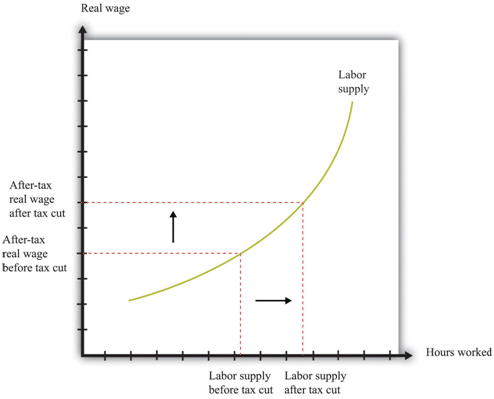
::图7:“劳动力对减税的供求反应”显示了减税的效果。如果劳动力供应曲线向上倾斜,减税会导致所供应劳动力数量的增加。如果劳动力供应增加,那么潜在产出也会增加。换句话说,减税的一个效果是促使人们更努力地工作并生产出更真实的GDP。为了保持简单,图8“劳动力对减税的供货反应”是假设由于减税而使实际工资的平衡没有变化。事实上,我们预计实际工资也会减少一些。劳动力的买主和卖主也会从减税中受益。 事实上,实际工资的减少促使企业购买个人希望提供的更多劳动力。 (如果我们将这一点列入我们的情况,那么税后实际工资还会增加,但比数字所显示的要少。 )- Figure 7: Labor Supply Response to Tax Cut
The wage that matters for labor supply decisions is the after-tax real wage. If income taxes are cut, and the real wage is unchanged, then households will supply more labor.
::劳动供给决定所必须的工资是税后实际工资。 如果削减所得税,而实际工资不变,那么家庭将提供更多劳动力。To view a Congressional Report on Tax Rates since 1945 visit .
::从1945年以来国会关于税率的报告访问。The Laffer Curve
::Laffer 曲线Supply-side economics was controversial and generated a great deal of debate back in the 1980s and since. Yet the argument that we have just presented is not really controversial at all. Almost all economists agreed that as a matter of theory, cuts in taxes could lead to increases in the quantity of labor supplied. The disagreements concerned the magnitude of the effect.
::供方经济学在1980年代和此后都颇具争议性,并引发了大量争论。 然而,我们刚才提出的论点根本没有真正争议。 几乎所有经济学家都同意,从理论上讲,减税可能导致劳动力供给量的增加。 分歧涉及影响的规模。Some proponents of supply-side economics made a much stronger claim. They said that the positive effects on labor supply could be so large that total tax revenues would increase, not decrease. They argued that even though the government would get less tax revenue on each dollar earned, people would work so much harder and generate so much more taxable income that the government would end up with more revenue than before.
::一些支持供方经济学的人提出了更强烈的要求。 他们说,对劳动力供给的积极影响可能很大,以至于税收总额会增加,而不是减少。 他们认为,即使政府获得的每美元税收收入会减少,人们也会更加努力地工作,创造更多的应纳税收入,最终政府的收入会比以前增加。This argument was encapsulated in the so-called Laffer curve. Economist Arthur Laffer asked what would happen if you graphed tax revenues as a function of the tax rate. Obviously (he observed) if the tax rate is zero, then tax revenues must be zero. And, Laffer argued, if the tax rate were 100 percent, so the government took every penny you earned, then no one would have an incentive to work at all, and the quantity of labor supplied would drop down to zero. Once again, income tax revenues would be zero. In between, tax revenues are positive. Figure 8: "Laffer Curve" shows an example of a Laffer curve. There is some tax rate that will lead to the maximum possible revenue for the government. This itself is not that interesting: the goal of the government is not to raise as much tax revenue as possible. But if the tax rate lies to the right of that point, then—as the picture shows—a cut in taxes will increase tax revenues.
::这一论点被概括在所谓的拉法尔曲线中。经济学家阿瑟·拉法尔询问,如果你将税收作为税率的函数来计算,会发生什么情况。显然(他观察过),如果税率为零,那么税收就必须为零。 拉法尔认为,如果税率为100%,那么政府就会拿走你赚到的每一分钱,那么没有人会有工作动力,劳动力数量就会下降到零。再次,所得税收入将是零。在两者之间,税收收入是正数。图8:“拉法尔曲线”显示了拉法尔曲线的一个例子。有些税率会导致政府获得尽可能最大的收入。这本身并不有趣:政府的目标不是要尽可能提高税收收入。但是,如果税率与该点的正确位置相同,那么——正如图所示——税收削减将增加税收收入。Figure 8: Laffer Curve
::图8:拉动曲线The Laffer curve says that it is possible for a reduction in the tax rate to lead to an increase in tax revenues. Although this is a theoretical possibility at very high tax rates, most economists view the Laffer curve as a theoretical curiosity with limited applicability to real economies.
::拉弗尔曲线指出,降低税率可能导致税收增加。 尽管在极高税率的情况下这是理论上的可能性,但大多数经济学家认为拉弗尔曲线是一种理论好奇,对实体经济的适用性有限。Just as almost all economists agreed that there would be some supply-side effects of income tax cuts, almost all economists agreed that the Laffer curve argument was inapplicable to the US economy (or indeed any other economy). The evidence indicated that the effects of tax cuts on hours worked were likely to be relatively small. Almost no economists actually believed that the economy was on the wrong side of the Laffer curve, where tax cuts could pay for themselves.
::正如几乎所有经济学家都同意所得税减税会有一些供应方效应一样,几乎所有经济学家都同意拉弗尔曲线观点不适用于美国经济(甚至任何其他经济体 ) 。 证据表明减税对工作时间的影响可能相对较小。 几乎没有经济学家实际认为经济在拉弗尔曲线的错误一边,减税可以为自己付出代价。Unfortunately, the Laffer curve argument was politically appealing, even though it was not supported by economic evidence. Buoyed by this argument, President Reagan oversaw both tax cuts and big increases in government spending. As a result, the US government ran large budget deficits. Following on from the ERTA, President Reagan and President George H. W. Bush after him were both forced to increase taxes to bring the budget back under control. The economic history of the United States in the 1980s was quite complex. Because this chapter concerns income taxes, we have considered only one of the policy changes of the Reagan administration. Other changes in tax policy were designed to promote savings. We have not discussed other aspects of President Reagan’s fiscal policy (there were large increases in government purchases), the tight monetary policy pursued by the Federal Reserve or the behavior of interest rates and exchange rates. All these are matters for other chapters.
::不幸的是,拉弗曲线论点在政治上颇具吸引力,尽管它没有得到经济证据的支持。 以这一论点为借口,里根总统监督了减税和政府开支的大幅增长。 结果,美国政府出现巨额预算赤字。 在埃塔、里根总统和乔治·W·布什总统之后,他被迫增加税收以重新控制预算。 1980年代美国的经济历史相当复杂。 由于这一章涉及所得税,我们只考虑里根政府的政策变化之一。 税收政策的其他变化是为了促进储蓄。 我们没有讨论里根总统财政政策的其他方面(政府采购大幅增长 ) 、 联邦储备所奉行的紧缩货币政策或利率和汇率的行为。 所有这些都是其他章节的问题。In Conclusion
::在结论结论中Our goal in this chapter was to understand the effects of tax changes on aggregate consumption and aggregate output. A tax cut puts more income in the hands of households, and thus consumption increases. The increase in consumption, in turn, leads to an expansion in the overall level of economic activity. The framework does a good job of describing and explaining actual economic outcomes during the Kennedy tax cut. We can thus have some faith that our basic framework is reasonably sound. Having said that, it is a very simple model that does have some deficiencies, most notably its neglect of the supply side of the economy.
::我们本章的目标是了解税收变化对总消费和总产出的影响。减税使更多的收入掌握在家庭手中,从而增加消费。消费的增加反过来又导致经济活动总体水平的扩大。这个框架很好地描述了和解释肯尼迪减税期间的实际经济结果。因此我们可以相信我们的基本框架是合理的。尽管如此,这是一个非常简单的模式,确实存在一些缺陷,特别是忽视了经济的供应方。Income tax cuts also decrease overall national saving. Income tax cuts increase household disposable income and lead to increased saving by households (as well as increased consumption). At the same time, however, income tax cuts mean that the government is saving less (or borrowing more). The net effect is to decrease national saving. The theory of economic growth tells us that reduced saving has the effect of decreasing future standards of living.
::收入减税也减少了国民储蓄总量,收入减税增加了家庭可支配收入,导致家庭储蓄增加(以及消费增加 ) 。 但与此同时,所得税减税意味着政府储蓄减少(或借贷增加 ) 。 净效果是减少国民储蓄。 经济增长理论告诉我们,储蓄减少会降低未来生活水平。We then examined the Reagan tax cuts of the 1980s. These tax cuts were aimed at stimulating employment and output by encouraging people to work more. The belief that tax cuts lead to an increase in the quantity of labor supplied is consistent with basic microeconomic principles, but there is disagreement about the likely size of the effect.
::接着我们审视了1980年代里根减税计划。 这些减税旨在通过鼓励人们更多工作来刺激就业和产出。 减税导致提供劳动力数量增加的信念符合基本的微观经济原则,但对效果的可能规模存在分歧。Although we cast our discussion of the effects of taxes on spending using the tax cuts of the Kennedy and Reagan administrations, the lesson is more general. It is common for the United States and other countries to use variations in income tax rates as a tool of intervention. We highlighted several effects of such interventions. Income tax changes alter the level of household disposable income and thus influence consumption expenditures; they affect saving and capital accumulation, and they affect labor supply. This policy tool, therefore, gives the government considerable influence on the aggregate economy.
::尽管我们讨论了税收对使用肯尼迪和里根政府减税措施进行支出的影响,但这一教训更为普遍。 美国和其他国家通常使用所得税税率的变动作为干预手段。 我们强调了这类干预措施的若干影响。 所得税的变动改变了家庭可支配收入水平,从而影响了消费支出;它们影响到储蓄和资本积累,并影响到劳动力供应。 因此,这一政策工具使政府对于总体经济产生了相当大的影响。Indeed, when the crisis of 2008 hit the world’s economies, many countries responded by implementing expansionary fiscal policies, including cuts in taxes. Australia, the United Kingdom, Singapore, Austria, and Brazil are just a few of the countries who cut taxes in response to the crisis.
::事实上,当2008年的危机冲击世界经济时,许多国家的反应是实施扩张性财政政策,包括减税。 澳大利亚、英国、新加坡、奥地利和巴西只是为应对危机而减税的少数国家。We used the Kennedy tax cut to illustrate demand-side effects and the Reagan tax cut to illustrate supply-side effects because those were the channels emphasized by the economic advisors at the time. Just about every change in the income tax code, however, has effects on consumption, saving, and labor supply. Every change in the code has short-run effects and long-run effects, and, as we have seen, these effects can be contradictory. Thus whenever you hear or read about proposed changes in taxes, you should try to remember that all these different stories will be in operation. The politicians and pundits who are supporting or opposing the change will typically talk about only one of them, depending on the spin they wish to convey. The analysis of this chapter should help you always see the bigger picture.
::我们用肯尼迪减税来说明需求方效应,用里根减税来说明供给方效应,因为这些是当时经济顾问们强调的渠道。不过,所得税法的每一个变化都会对消费、储蓄和劳动力供应产生影响。守则的每一个变化都有短期效应和长期效应,而且正如我们所看到的那样,这些效应可能相互矛盾。因此,每当你听到或阅读税收的拟议变化时,你应该尽量记住所有这些不同的故事都会在起作用。支持或反对这些变化的政治家和专家通常只谈论其中的一个,取决于他们想要传达的旋律。对本章的分析应该有助于你永远看到更大的画面。Finally, remember that tax changes will typically have major effects on the distribution of income. There are winners and losers from every change in the tax code. This, above all, is why changes in the tax code are an endless source of political debate.
::最后,请记住,税收变化通常会对收入分配产生重大影响。 税法的每一次变化都有赢家和输家。 这首先是为什么税法的改变是政治辩论无休止的源头。To view current issues visit the .
::观察目前的问题访问。Key Takeaways on Kennedy
::肯尼迪的关键外卖-
Beginning in the early 1960s, the growth of real GDP began to slow. This provided the basis for the tax cut of 1964.
::从1960年代初开始,实际国内生产总值的增长开始放缓,为1964年减税提供了基础。 -
The CEA economists used the aggregate expenditure model as the basis for their analysis of the effects of the tax cut.
::CEA经济学家以总开支模式作为分析减税影响的基础。 -
In response to the tax cut, consumption and real GDP both increased. This fits with the prediction of the aggregate expenditure model.
::由于减税,消费和实际国内生产总值都有所增加,这符合对总支出模式的预测。 -
Since the marginal propensity to consume is less than 1, a tax cut will lead to a household to consume more and save more.
::由于边际消费倾向小于1,减税将导致家庭消费更多、储蓄更多。 -
National savings, the sum of public and private savings, will generally decrease when there is a tax cut.
::国民储蓄,即公共和私人储蓄的总和,在减税时一般会减少。
Key Takeaways on Reagan
::Reagan 上的 Key 外卖-
Prior to the Reagan tax cut, the US economy was experiencing both low growth in real GDP and high inflation.
::在里根减税之前,美国经济既经历了实际国内生产总值低增长,又经历了高通胀。 -
Reagan’s economic advisors stressed the effects of taxes on the supply side of the economy, and in particular the incentive effects of taxes on labor supply and investment.
::Reagan的经济顾问强调了税收对经济供应方的影响,特别是税收对劳动力供应和投资的刺激作用。 -
The Reagan tax cuts led to considerably higher deficits in the United States.
::里根减税导致美国赤字大幅上升。
Answer the self check questions below to monitor your understanding of the concepts in this section.
::回答下面的自我核对问题,以监测你对本节概念的理解。Self Check Questions
::自查问题1. What matters for labor supply decisions - the marginal tax rate or the average tax rate?
::1. 劳动力供应决定涉及什么事项 -- -- 边际税率或平均税率?2. According to the Laffer curve, does a tax cut always increase tax revenues?
::2. 根据拉弗尔曲线,减税是否总是增加税收?3. What was the state of the economy at the time of the Reagan tax cut?
::3. 里根减税时的经济状况如何?4. What framework was used for analyzing the effects of the Reagan tax cut?
::4. 在分析里根减税的影响时采用了何种框架?5. What were the effects of the Reagan tax cut?
::5. 里根减税有何影响?6. Go to the Bureau of Economic Analysis website. Visit the section on . Examine what has happened recently to personal income and disposable income. Have they been increasing or decreasing? How does this affect you?
::6. 请访问经济分析局网站,查阅关于最近个人收入和可支配收入的情况,这些收入在增加还是减少?这对你有何影响?7. Pick a country other than the United States. Can you find income tax rates for that country? How do they compare to the United States?
::7. 选择美国以外的国家。你能找到美国的所得税率吗?这些税率与美国相比如何?8. Go to the IRS webpage. Suppose that you are a member of a married household with a total income of $55,000. What are your marginal and average tax rates? Compare those to the tax rates on individuals. Which group faces the higher marginal income tax rate?
::8. 前往国税局网页,假设你是一个已婚家庭的成员,总收入为55,000美元,你的边际税率和平均税率是多少?与个人税率比较,哪个群体面临较高的边际所得税率?9. In the summer of 2010, the George W. Bush tax cuts were about to expire. What would the change in the tax rates be if tax cuts had been allowed to expire?
::9. 2010年夏季,乔治·布什的减税即将到期,如果允许减税期满,税率的变化会如何?10. Go online and research the current tax situation under the Trump administration. What are the criticisms of the current tax situation?
::10. 上网研究特朗普政府当前的税收状况,对当前税收状况有何批评?
-
The consequence of tax reform was to make the individual tax code more complex than ever.