机器学习
一种人工神经网络(ANN)系统基于一种称为感知器的单元,如下图所示。感知器接收一个实值输入向量,计算这些输入的线性组合,然后如果结果大于某个阈值则输出 1,否则输出 -1。更精确地说,给定输入 x1 到 xn,感知器计算的输出 o(x1,...,xn) 为:
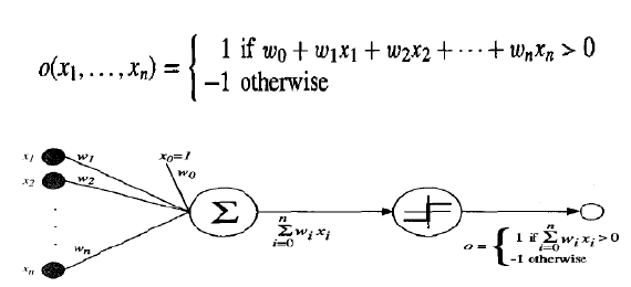
其中每个 wi 是一个实值常数或权重,它决定了输入 xi 对感知器输出的贡献。注意,量 (−w0) 是一个阈值,加权输入组合 必须超过这个阈值,感知器才能输出 1。
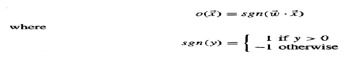
为了简化表示,我们设有一个额外的常数输入 ,这使得我们可以将上述不等式写作 ,或者以向量形式写作 。为简洁起见,我们有时将感知器函数写作 。
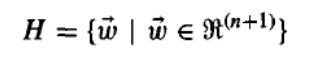
学习一个感知器涉及为权重 w0,...,wn 选择值。因此,感知器学习中考虑的候选假设空间 H 是所有可能的实值权重向量的集合。
感知器的表示能力:
我们可以将感知器视为在 n 维空间中表示一个超平面决策面,并对位于另一侧的实例输出 -1,如下图所示。这个决策超平面的方程是 。当然,有些正例和负例的集合不能被任何超平面分开。那些可以被分开的集合称为线性可分示例集。
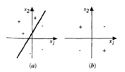
两输入感知器表示的决策面。(a) 一组训练示例和一个正确分类它们的感知器的决策面。(b) 一组非线性可分的训练示例(即不能被任何直线正确分类的示例)。x1 和 x2 是感知器输入。正例用“+”表示,负例用“-”表示。输入被送入多个单元,这些单元的输出再作为第二级(最终级)的输入。一种方法是以析取范式表示布尔函数(即作为输入及其非的合取(AND)集合的析取(OR))。请注意,AND 感知器的输入可以通过简单地改变相应输入权重的符号来取反。因为阈值单元网络可以表示各种丰富的函数,而单个单元本身不能,所以我们通常会对学习多层阈值单元网络感兴趣。
感知器训练规则
尽管我们对学习许多相互连接单元的网络感兴趣,但让我们首先了解如何学习单个感知器的权重。这里的精确学习问题是确定一个权重向量,使得感知器对每个给定的训练示例产生正确的 ±1 输出。
已知有几种算法可以解决这个学习问题。这里我们考虑两种:感知器规则和 Delta 规则。这两种算法在不同的条件下,保证收敛到一些不同的可接受假设。它们对人工神经网络很重要,因为它们为学习许多单元的网络提供了基础。
学习可接受权重向量的一种方法是从随机权重开始,然后迭代地将感知器应用于每个训练示例,当它错误分类一个示例时修改感知器权重。这个过程重复进行,根据需要多次迭代训练示例,直到感知器正确分类所有训练示例。权重在每一步都根据感知器训练规则进行修改,该规则根据以下规则修正与输入 xi 关联的权重 wi:
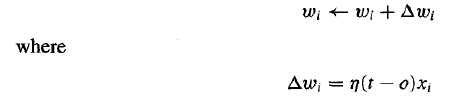
其中 t 是当前训练示例的目标输出,o 是感知器生成的输出,η 是一个称为学习率的正数常数。学习率的作用是调节每一步权重改变的程度。它通常设置为某个小值(例如 0.1),有时会随着权重调整迭代次数的增加而衰减。
为什么这个更新规则会收敛到成功的权重值?为了获得直观的感觉,考虑一些具体情况。假设训练示例已经被感知器正确分类。在这种情况下, 为零,使得 Δwi 为零,因此没有权重被更新。假设感知器输出 -1,而目标输出是 +1。为了在这种情况下使感知器输出 +1 而不是 -1,必须改变权重以增加 的值。例如,如果 ,那么增加 wi 将使感知器更接近正确分类这个示例。注意,在这种情况下,训练规则将增加 wi,因为 、η 和 xi 都为正。例如,如果 ,那么权重更新将是 。另一方面,如果 且 ,那么与正 xi 相关的权重将减少而不是增加。
实际上,可以证明上述学习过程在感知器训练规则的有限次应用内收敛到一个正确分类所有训练示例的权重向量,前提是训练示例是线性可分的并且使用了足够小的 η。如果数据不是线性可分的,则不保证收敛。
梯度下降和 Delta 规则
尽管感知器规则在训练示例线性可分时可以找到一个成功的权重向量,但如果示例不是线性可分,它可能会无法收敛。第二种训练规则,称为 Delta 规则,旨在克服这个困难。如果训练示例不是线性可分,Delta 规则会收敛到目标概念的最佳拟合近似。Delta 规则背后的关键思想是使用梯度下降来搜索可能的权重向量的假设空间,以找到最适合训练示例的权重。这个规则很重要,因为梯度下降为 反向传播算法(BACKPROPAGATION algorithm) 提供了基础,该算法可以学习具有许多相互连接单元的网络。它也很重要,因为梯度下降可以作为需要搜索包含许多不同类型连续参数化假设的假设空间的学习算法的基础。
Delta 训练规则最好通过考虑训练无阈值感知器的任务来理解;也就是说,一个线性单元,其输出 o 由下式给出:
因此,线性单元对应于感知器的第一阶段,没有阈值。
为了推导线性单元的权重学习规则,我们首先指定一个度量来衡量假设(权重向量)相对于训练示例的训练误差。尽管有许多方法可以定义这个误差,但一个常用的且特别方便的度量是:
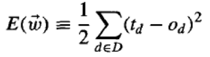
其中 D 是训练示例集,td 是训练示例 d 的目标输出,od 是线性单元对训练示例 d 的输出。根据这个定义,E(w ) 简单来说就是目标输出 td 和线性单元输出 od 之间差的平方的一半,对所有训练示例求和。这里我们将 E 描述为 w 的函数,因为线性单元输出 o 取决于这个权重向量。当然,E 也取决于特定的训练示例集,但我们假设这些在训练期间是固定的,因此我们不费心将 E 显式地写成这些的函数。特别是,我们在这里证明,在某些条件下,使 E 最小化的假设也是在给定训练数据下 H 中最可能的假设。
One type of ANN system is based on a unit called a perceptron, illustrated in below Figure: A
perceptron takes a vector of real-valued inputs, calculates a linear combination of these inputs, then
outputs a 1 if the result is greater than some threshold and -1 otherwise. More precisely, given inputs xl
through xn the output o(xl, . . . , xn) computed by the perceptron is
where each
w i
is a real-valued constant, or weight, that determines the contribution of input xi
to
the perceptron output. Notice the quantity ( w 0
) is a threshold that the weighted combination of
inputs w 1
x 1
.... w n
x n
must surpass in order for the perceptron to output a 1.
To simplify notation, we imagine an additional constant input
x0
1 , allowing us to write the above
inequality as
n
i 0
w i
xi
0 , or in vector form as w. x o . For brevity, we will sometimes write the
perceptron function as
Learning a perceptron involves choosing values for the weights
w 0
,...., w n
Therefore, the space H of
candidate hypotheses considered in perceptron learning is the set of all possible real-valued weight
vectors.
Representational Power of Perceptrons:
We can view the perceptron as representing a hyperplane decision surface in the n--dimensional spacand outputs a -1 for instances lying on the other side, as illustrated in Figure below The equation for this
decision hyperplane is w. x 0 . Of course, some sets of positive and negative examples cannot be
separated by any hyperplane. Those that can be separated are called linearly separable sets of
examples.
The decision surface represented by a two-input perceptron. (a) A set of training examples and
the decision surface of a perceptron that classifies them correctly. (b) A set of training examples that is
not linearly separable (i.e., that cannot be correctly classified by any straight line). xl and x2 are the
Perceptron inputs. Positive examples are indicated by "+", negative by "-". The inputs are fed to multiple
units, and the outputs of these units are then input to a second, final stage. One way is to represent the
Boolean function in disjunctive normal form (i.e., as the disjunction (OR) of a set of conjunctions (ANDs)
of the inputs and their negations). Note that the input to an AND perceptron can be negated simply by
changing the sign of the corresponding input weight. Because networks of threshold units can represent
a rich variety of functions and because single units alone cannot, we will generally be interested in
learning multilayer networks of threshold units.
The Perceptron Training Rule
Although we are interested in learning networks of many interconnected units, let us begin by
understanding how to learn the weights for a single perceptron. Here the precise learning problem is to
determine a weight vector that causes the perceptron to produce the correct 1 output for each of the
given training examples.
Several algorithms are known to solve this learning problem. Here we consider two: the
perceptron rule and the delta rule. These two algorithms are guaranteed to converge to somewhat
different acceptable hypotheses, under somewhat different conditions. They are important to ANNs
because they provide the basis for learning networks of many units.
One way to learn an acceptable weight vector is to begin with random weights, then iteratively
apply the perceptron to each training example, modifying the perceptron weights whenever it
misclassifies an example. This process is repeated, iterating through the training examples as many
times as needed until
the perceptron classifies all training examples correctly. Weights are modified at each step according to
the perceptron training rule, which revises the weight wi associated with input xi according to the rule
Here t is the target output for the current training example, o is the output generated by the
46
perceptron, and is a positive constant called the learning rate. The role of the learning rate is to
moderate the degree to which weights are changed at each step. It is usually set to some small value
(e.g., 0.1) and is sometimes made to decay as the number of weight-tuning iterations increases.
Why should this update rule converge toward successful weight values? To get an intuitive feel,
consider some specific cases. Suppose the training example is correctly classified already by the
perceptron. In this case, (t - o) is zero, making w
i zero, so that no weights are updated. Suppose the
perceptron outputs a -1, when the target output is +1. To make the perceptron output a+1 instead of -1
in this case, the weights must be altered to increase the value of w. x For example, if xi>0, then
increasing wi will bring the perceptron closer to correctly classifying this example. Notice the training
rule will increase w, in this case, because (t - o), , and xi are all positive. For example, if xi = .8, = 0.1,
t = 1, and o = - 1, then the weight update will be
w i
= (t - o)xi
= O.1(1 - (-1))0.8 = 0.16. On the
other hand, if t = -1 and o = 1, then weights associated with positive xi will be decreased rather than
increased.
In fact, the above learning procedure can be proven to converge within a finite number of applications
of the perceptron training rule to a weight vector that correctly classifies all training examples, provided
the training examples are linearly separable and provided a sufficiently small is used. If the data are
not linearly separable, convergence is not assured.
Gradient Descent and the Delta Rule
Although the perceptron rule finds a successful weight vector when the training examples are
linearly separable, it can fail to converge if the examples are not linearly separable. A second training
rule, called the delta rule, is designed to overcome this difficulty. If the training examples are not
linearly separable, the delta rule converges toward a best-fit approximation to the target concept. The
key idea behind the delta rule is to use gradient descent to search the hypothesis space of possible
weight vectors to find the weights that best fit the training examples. This rule is important because
gradient descent provides the basis for the BACKPROPAGATION algorithm, which can learn networks
with many interconnected units. It is also important because gradient descent can serve as the basis for
learning algorithms that must search through hypothesis spaces containing many different types of
continuously parameterized hypotheses.
The delta training rule is best understood by considering the task of training an unthresholded
perceptron; that is, a linear unit for which the output o is given by
Thus, a linear unit corresponds to the first stage of a perceptron, without the threshold.
In order to derive a weight learning rule for linear units, let us begin by specifying a measure for the
training error of a hypothesis (weight vector), relative to the training examples. Although there are
many ways to define this error, one common measure that will turn out to be especially convenient is
where D is the set of training examples, td is the target output for training example d, and od is the
output of the linear unit for training example d. By this definition, E w
is simply half the squared
47
difference between the target output td and the hear unit output od , summed over all training
examples. Here we characterize E as a function of w
, because the linear unit output o depends on this
weight vector. Of course E also depends on the particular set of training examples, but we assume these
are fixed during training, so we do not bother to write E as an explicit function of these. In particular,
there we show that under certain conditions the hypothesis that minimizes E is also the most probable
hypothesis in H given the training data.