机器学习
组合多个分类器最简单的方法是投票法(Voting),它对应于对学习器进行线性组合,参见图 1。
这也称为集成(ensembles)和线性意见池(linear opinion pools)。在最简单的情况下,所有学习器都被赋予相同的权重,我们进行简单投票,这相当于取平均值。尽管如此,取(加权)和只是可能性之一,还有其他组合规则,如表 1 所示。如果输出不是后验概率,这些规则要求将输出归一化到相同的尺度。
表 1 - 分类器组合规则
| 规则 | 公式 |
| 求和 (Sum) | |
| 乘积 (Product) | |
| 最小 (Min) | |
| 最大 (Max) | |
| 中位数 (Median) |
这些规则的使用示例显示在表 2 中,该表演示了不同规则的效果。求和规则是最直观的,也是实践中使用最广泛的。中位数规则对异常值更鲁棒;最小规则和最大规则分别悲观和乐观。使用乘积规则时,每个学习器都具有否决权;无论其他学习器如何,如果一个学习器的输出为 0,则整体输出变为 0。请注意,在组合规则之后,yi 不一定总和为 1。
表 2:三个学习器和三个类别上的组合规则示例
| 学习器 | 类 C1 | 类 C2 | 类 C3 |
| M1 | 0.9 | 0.1 | 0.0 |
| M2 | 0.8 | 0.2 | 0.0 |
| M3 | 0.0 | 0.9 | 0.1 |
| 求和 | 1.7 | 1.2 | 0.1 |
| 乘积 | 0.0 | 0.0 | 0.0 |
| 最小 | 0.0 | 0.1 | 0.0 |
| 最大 | 0.9 | 0.9 | 0.1 |
| 中位数 | 0.8 | 0.2 | 0.0 |
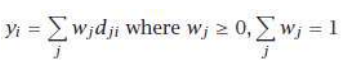
在加权求和中,dji 是学习器 j 对类别 Ci 的投票,wj 是其投票的权重。简单投票是一种特殊情况,其中所有投票者具有相同的权重,即 。在分类中,这被称为多数投票法(plurality voting),其中获得最多票数的类别获胜。
当只有两个类别时,这就是多数表决(majority voting),获胜类别获得超过一半的票数。如果投票者还可以提供他们对每个类别的投票程度的附加信息(例如,通过后验概率),那么在归一化之后,这些信息可以用作加权投票方案中的权重。等效地,如果 dji 是类后验概率 P(Ci∣x,Mj),那么我们只需将它们相加 () 并选择具有最大 yi 的类别。
在回归的情况下,可以使用简单或加权平均值或中位数来融合基回归器的输出。中位数比平均值对噪声更鲁棒。
寻找 wj 的另一种可能方法是在单独的验证集上评估学习器(回归器或分类器)的准确性,并使用该信息来计算权重,以便我们给予更准确的学习器更大的权重。
投票方案可以被视为贝叶斯框架下的近似,其中权重近似先验模型概率,模型决策近似模型条件似然。
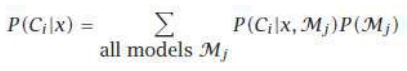
简单投票对应于均匀先验。如果我们有一个偏向简单模型的先验分布,这将赋予它们更大的权重。我们不能对所有模型进行积分;我们只选择我们认为 P(Mj) 较高的子集,或者我们可以进行另一个贝叶斯步骤,计算 P(Ci∣x,Mj)(给定样本的模型概率),并从该密度中抽样高概率模型。
让我们假设 dj 是独立同分布的(iid),期望值为 E[dj],方差为 Var(dj)。那么当我们使用 进行简单平均时,输出的期望值和方差为:
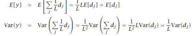
我们看到期望值没有改变,所以偏差没有改变。但方差(以及均方误差)随着独立投票者数量 L 的增加而减小。在一般情况下:
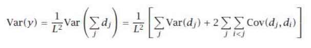
这意味着如果学习器正相关,方差(和误差)会增加。因此,我们可以将使用不同算法和输入特征视为努力减少(如果不能完全消除)正相关。
The simplest way to combine multiple classifiers is by voting, which corresponds to taking a
linear combination of the learn
ers, Refer figure 1.
This is also known as ensembles and linear opinion pools. In the sim plest case, all learners are
given equal weight and we have simple voting that corresponds to taking an average. Still, taking a
(weighted) sum is only one of the possibilities and there are also other combination rules, as shown in
table 1. If the outputs are not posterior probabilities, these rules require that outputs be normalized to
the same scale
Table 1 - Classifier combination rules
An example of the use of these rules is shown in table 2, which demonstrates the effects of
different rules. Sum rule is the most intuitive and is the most widely used in practice. Median rule is
more robust to outliers; minimum and maximum rules are pessimistic and optimistic, respectively. With
the product rule, each learner has veto power; regardless of the other ones, if one learner has an
output of 0, the overall output goes to 0. Note that after the combination rules, yi do not necessarily
sum up to 1.
Table 2: Example of combination rules on three learners and three classes
In weighted sum, dji is the vote of learner j for class Ci and wj is the weight of its vote. Simple voting is a
special case where all voters have equal weight, namely, wj = 1/L. In classification, this is called plurality
voting where the class having the maximum number of votes is the winner.
When there are two classes, this is majority voting where the winning class gets more than half of the
votes. If the voters can also supply the additional information of how much they vote for each class
(e.g., by the posterior probability), then after normalization, these can be used as weights in a weighted
voting scheme. Equivalently, if dji are the class posterior probabilities, P(Ci | x,Mj ), then we can just sum
them up (wj = 1/L) and choose the class with maximum yi .
In the case of regression, simple or weighted averaging or median can be used to fuse the outputs of
base-regressors. Median is more robust to noise than the average.
Another possible way to find wj is to assess the accuracies of the learners (regressor or classifier) on a
separate validation set and use that information to compute the weights, so that we give more weights
to more accurate learners.
Voting schemes can be seen as approximations under a Bayesian framework with weights
approximating prior model probabilities, and model decisions approximating model-conditional
likelihoods.
Simple voting corresponds to a uniform prior. If we have a prior distribution preferring simpler models,
this would give larger weights to them. We cannot integrate over all models; we only choose a subset
for which we believe P(Mj ) is high, or we can have another Bayesian step and calculate P(Ci | x,Mj ), the
probability of a model given the sample, and sample high probable models from this density.
Let us assume that dj are iid with expected value E[dj] and variance Var(dj ), then when we take a simple
63
average with wj = 1/L, the expected value and variance of the output are
We see that the expected value does not change, so the bias does not change. But variance, and
therefore mean square error, decreases as the number of independent voters, L, increases. In the
general case,
which implies that if learners are positively correlated, variance (and error) increase. We can thus view
using different algorithms and input features as efforts to decrease, if not completely eliminate, the
positive correlation.