机器学习
随机森林(Random Forest) 是一种集成学习方法,它构建多棵决策树,然后将它们合并起来以获得更准确的预测。
如果在机器学习中有一种方法在过去几年中越来越受欢迎,那就是随机森林的概念。这个概念已经存在了更长时间,有几位不同的人发明了各种变体,但与它联系最紧密的名字是 Breiman,他也在第二单元中描述了 CART 算法。
图 3:多数投票的随机森林示例
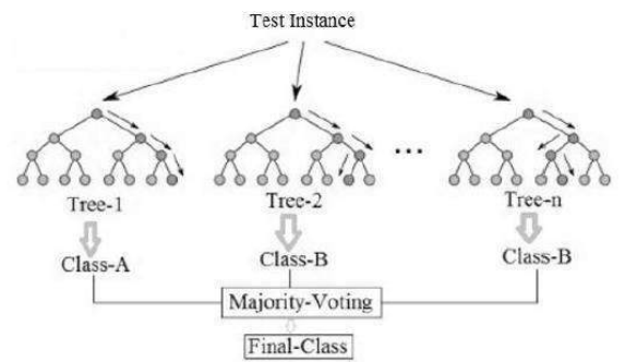
其核心思想是,如果一棵树是好的,那么许多树(一片森林)应该会更好,前提是它们之间有足够的多样性。随机森林最有趣的地方在于它从标准数据集中创建随机性的方式。它使用的第一种方法就是我们刚刚看到的:Bagging(自举聚合)。如果我们想创建一片森林,我们可以通过在稍微不同的数据上训练每棵树来使它们不同,所以我们从数据集中为每棵树抽取自举样本。
然而,这还不足以产生足够的随机性。另一个可以添加随机性的明显地方是限制决策树可以做出的选择。在每个节点处,将特征的一个随机子集提供给树,它只能从该子集中进行选择,而不是从整个集合中进行选择。这不仅增加了每棵树训练中的随机性,还加快了训练速度,因为在每个阶段需要搜索的特征更少。当然,它引入了一个新的参数(要考虑多少特征),但随机森林似乎对这个参数不是很敏感;实际上,子集大小是特征数量的平方根似乎很常见。这两种形式的随机性作用是减少方差而不影响偏差。另一个好处是无需修剪树。还有一个我们还不知道如何选择的参数,那就是森林中树的数量。然而,如果想要获得最佳结果,这很容易选择:我们可以持续构建树,直到误差不再减小。
一旦训练好这组树,森林的输出就是分类的多数投票(与我们见过的其他委员会方法一样),或者是回归的平均响应。这些基本上就是创建随机森林所需的主要特征。在看到随机森林的一些结果之前,下面给出了该算法。
算法
以下是随机森林算法的概要。
- 随机森林算法生成许多分类树。每棵树的生成方式如下: a) 如果训练集中的示例数量为 N,则从原始数据中随机(有放回地)抽取 N 个示例。此样本将作为生成树的训练集。 b) 如果有 M 个输入变量,则指定一个数字 m,使得在每个节点处,从 M 个变量中随机选择 m 个变量,并使用这 m 个变量上的最佳分割来分割节点。在森林中生成各种树的过程中,m 的值保持不变。 c) 每棵树都尽可能地生长到最大程度。
- 要从输入向量对新对象进行分类,请将输入向量放入森林中的每棵树中。每棵树都会给出一个分类,我们说这棵树为该类别“投票”。森林选择具有最多投票的类别。
该算法的实现非常简单:我们修改决策树以接受一个额外的参数 m,即每个阶段选择集中应使用的特征数量。我们很快将通过一个示例来了解其用法,并与 Boosting 进行比较。
查看算法,您可能会发现它是一种非常不寻常的机器学习方法,因为它具有**“尴尬的并行性”(embarrassingly parallel):由于树之间不相互依赖,如果您有多个处理器,则可以在不同的独立处理器上同时创建和获取不同树的决策。这意味着随机森林可以在您拥有的任意数量的处理器上运行,并且几乎可以实现线性加速**。
关于随机森林,还有一件值得一提的好处,那就是只需少量编程工作,它们就带有内置的测试数据:自举样本平均会遗漏大约 35% 的数据,即所谓的袋外(out-of-bootstrap)示例。如果我们跟踪这些数据点,那么它们可以作为该特定树的新样本,从而在不使用任何额外数据点的情况下获得估计的测试误差。
这避免了交叉验证的需要。
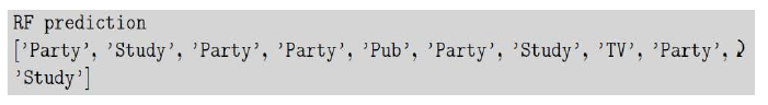
作为一个使用随机森林的简短示例,我们首先演示随机森林在本次和前几章中使用的 Party 示例上获得了正确的结果,该示例基于 10 棵树,每棵树在 7 个样本上训练,并且每棵树最多允许两层:
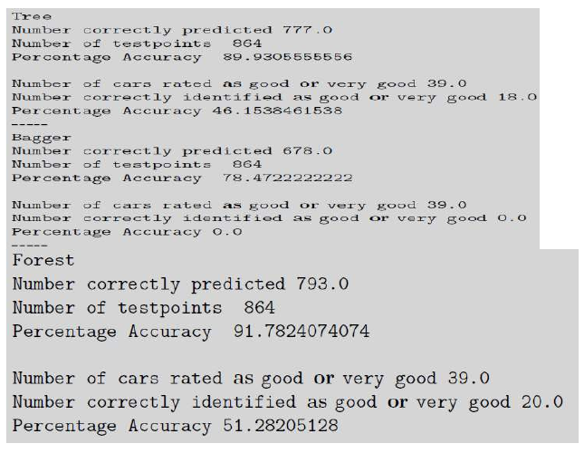
作为一个更复杂的例子,UCI 存储库中的汽车评估数据集包含 1,728 个示例,旨在根据六个属性分类汽车是否值得购买。以下结果比较了单个决策树、Bagging 以及包含 50 棵树的随机森林,每棵树基于 100 个样本,且每棵树的最大深度为五。可以看出,随机森林是这三种方法中最准确的。
优点和缺点
优点
以下是随机森林的一些重要优点。
- 它在大型数据库上高效运行。
- 它可以处理数千个输入变量而无需变量删除。
- 它能估计哪些变量在分类中很重要。
- 它具有估计缺失数据的有效方法,并且在大量数据缺失时仍能保持准确性。
- 生成的森林可以保存以供将来在其他数据上使用。
- 计算出原型(Prototypes),提供变量与分类之间关系的信息。
- 上述功能可以扩展到未标记数据,从而实现无监督聚类、数据视图和异常检测。
- 它提供了一种检测变量交互的实验方法。
- 随机森林的运行时间相当快,并且能够处理不平衡和缺失的数据。
- 它们可以处理二元特征、类别特征、数值特征,而无需任何缩放。
缺点
- 随机森林算法的一个缺点是,当用于回归时,它们无法预测训练数据范围之外的值,并且它们可能过度拟合特别嘈杂的数据集。
- 随机森林创建的模型大小可能非常大。它可能占用数百兆字节的内存,并且评估速度可能很慢。
- 随机森林模型是黑箱,很难解释。
A random forest is an ensemble learning method where multiple decision trees are constructed
and then they are merged to get a more accurate prediction.
If there is one method in machine learning that has grown in popularity over the last few years,
then it is the idea of random forests. The concept has been around for longer than that, with several
different people inventing variations, but the name that is most strongly attached to it is that of
Breiman, who also described the CART algorithm in unit 2.
Figure 3: Example of random forest with majority voting
The idea is largely that if one tree is good, then many trees (a forest) should be better, provided
that there is enough variety between them. The most interesting thing about a random forest is the
ways that it creates randomness from a standard dataset. The first of the methods that it uses is the
one that we have just seen: bagging. If we wish to create a forest then we can make the trees different
by training them on slightly different data, so we take bootstrap samples from the dataset for each tree.
However, this isn’t enough randomness yet. The other obvious place where it is possible to add
randomness is to limit the choices that the decision tree can make. At each node, a random subset of
the features is given to the tree, and it can only pick from that subset rather than from the whole set.
As well as increasing the randomness in the training of each tree, it also speeds up the training,
since there are fewer features to search over at each stage. Of course, it does introduce a new
parameter (how many features to consider), but the random forest does not seem to be very sensitive
to this parameter; in practice, a subset size that is the square root of the number of features seems to
be common. The effect of these two forms of randomness is to reduce the variance without effecting
the bias. Another benefit of this is that there is no need to prune the trees. There is another parameter
that we don’t know how to choose yet, which is the number of trees to put into the forest. However,
this is fairly easy to pick if we want optimal results: we can keep on building trees until the error stops
decreasing.
Once the set of trees are trained, the output of the forest is the majority vote for classification,
as with the other committee methods that we have seen, or the mean response for regression. And
those are pretty much the main features needed for creating a random forest. The algorithm is given
next before we see some results of using the random forest.
Algorithm
Here is an outline of the random forest algorithm.
1. The random forests algorithm generates many classification trees. Each tree is generated as
follows:
a) If the number of examples in the training set is N, take a sample of N examples at
random - but with replacement, from the original data. This sample will be the training
set for generating the tree.
b) If there are M input variables, a number m is specified such that at each node, m
variables are selected at random out of the M and the best split on these m is used to
68
2.split the node. The value of m is held constant during the generation of the various
trees in the forest.
c) Each tree is grown to the largest extent possible.
To classify a new object from an input vector, put the input vector down each of the trees in the
forest. Each tree gives a classification, and we say the tree “votes” for that class. The forest
chooses the classification
The implementation of this is very easy: we modify the decision to take an extra parameter, which is m,
the number of features that should be used in the selection set at each stage. We will look at an
example of using it shortly as a comparison to boosting.
Looking at the algorithm you might be able to see that it is a very unusual machine learning
method because it is embarrassingly parallel: since the trees do not depend upon each other, you can
both create and get decisions from different trees on different individual processors if you have them.
This means that the random forest can run on as many processors as you have available with nearly
linear speedup.
There is one more nice thing to mention about random forests, which is that with a little bit of
programming effort they come with built-in test data: the bootstrap sample will miss out about 35% of
the data on average, the so-called out-of-bootstrap examples. If we keep track of these datapoints then
they can be used as novel samples for that particular tree, giving an estimated test error that we get
without having to use any extra datapoints.
This avoids the need for cross-validation.
As a brief example of using the random forest, we start by demonstrating that the random
forest gets the correct results on the Party example that has been used in both this and the previous
chapters, based on 10 trees, each trained on 7 samples, and with just two levels allowed in each tree:
As a rather more involved example, the car evaluation dataset in the UCI Repository contains 1,728
examples aiming to classify whether or not a car is a good purchase based on six attributes. The
following results compare a single decision tree, bagging, and a random forest with 50 trees, each based
on 100 samples, and with a maximum depth of five for each tree. It can be seen that the random forest
is the most accurate of the three methods.
69
Strengths and weaknesses
Strengths
The following are some of the important strengths of random forests.
• It runs efficiently on large data bases.
• It can handle thousands of input variables without variable deletion.
• It gives estimates of what variables are important in the classification.
• It has an effective method for estimating missing data and maintains accuracy when a large
proportion of the data are missing.
• Generated forests can be saved for future use on other data.
• Prototypes are computed that give information about the relation between the variables and the
classification.
• The capabilities of the above can be extended to unlabeled data, leading to unsupervised
clustering, data views and outlier detection.
• It offers an experimental method for detecting variable interactions.
• Random forest run times are quite fast, and they are able to deal with unbalanced and missing
data.
• They can handle binary features, categorical features, numerical features without any need for
scaling.
Weaknesses
•
A weakness of random forest algorithms is that when used for regression they cannot predict
beyond the range in the training data, and that they may over-fit data sets that are particularly
noisy.
70
•
•
The sizes of the models created by random forests may be very large. It may take hundreds of
megabytes of memory and may be slow to evaluate.
Random forest models are black boxes that are very hard to interpret.