机器学习
然而,假设我们有相同的数据,但没有目标标签。这需要无监督学习。假设不同的类别各自来自它们自己的高斯分布。这被称为多模态数据,因为每个不同的类别都有一个分布(模式)。我们不能用一个高斯分布来拟合数据,因为它整体上看起来不像高斯分布。
但是,我们可以做一些事情。如果我们知道数据中有多少个类别,那么我们可以一次性估计那么多高斯分布的参数。如果我们不知道,那么我们可以尝试不同的数量,看看哪个效果最好。我们将在第二单元中讨论另一种方法(k-means 算法)的这个问题。完全可以使用任何其他概率分布而不是高斯分布,但高斯分布是迄今为止最常见的选择。
那么,输入到算法的任何特定数据点的输出将是所有 M 个高斯分布所期望值的总和:
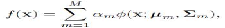
其中 N(x;μm,Σm) 是一个均值为 μm 和协方差矩阵为 Σm 的高斯函数,而 αm 是权重,约束条件是 。
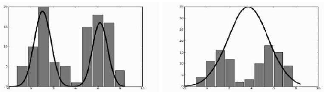
图 4 显示了两个示例,其中数据(由直方图显示)来自两个不同高斯分布,并且模型被计算为两个高斯分布的总和或混合。
图 4:来自两个高斯分布混合的训练数据直方图和两个拟合模型,显示为线图。左侧显示的模型拟合得很好,但右侧的模型产生了两个几乎重叠的高斯分布,与数据拟合不佳。
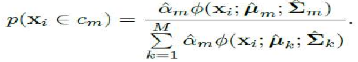
该图也为您提供了一些关于一旦创建了混合模型如何使用的想法。输入 xi 属于类别 m 的概率可以写成(变量上的帽子 (⋅^) 表示我们正在估计该变量的值):
问题在于如何选择权重 αm。常见的方法是旨在找到最大似然解(似然是给定模型的数据的条件概率,最大似然解通过改变模型来最大化这个条件概率)。实际上,通常会计算对数似然然后最大化它;它保证是负值,因为概率都小于 1,并且对数会展开值,使优化更有效。所使用的算法是期望-最大化 (Expectation-Maximization,简称 EM) 算法的一个非常通用的示例。
However, suppose that we have the same data, but without target labels. This requires
unsupervised learning, Suppose that the different classes each come from their own Gaussian
distribution. This is known as multi-modal data, since there is one distribution (mode) for each different
class. We can’t fit one Gaussian to the data, because it doesn’t look Gaussian overall.
There is, however, something we can do. If we know how many classes there are in the data,
then we can try to estimate the parameters for that many Gaussians, all at once. If we don’t know, then
we can try different numbers and see which one works best. We will talk about this issue more for a
different method (the k-means algorithm) in Unit 2. It is perfectly possible to use any other probability
distribution instead of a Gaussian, but Gaussians are by far the most common choice. Then the output
for any particular datapoint that is input to the algorithm will be the sum of the values expected by all
of the M Gaussians:
where _(x ; μm, m) is a Gaussian function with mean μm and covariance matrix
weights with the constraint that M
m =1 αm =1.
m, and the αm are
The given figures 4 shows two examples, where the data (shown by the histograms) comes from two
different Gaussians, and the model is computed as a sum or mixture of the two Gaussians together.
FIGURE 4: Histograms of training data from a mixture of two Gaussians and two fitted models, shown as
the line plot. The model shown on the left fits well, but the one on the right produces two Gaussians
right on top of each other that do not fit the data well.
The figure also gives you some idea of how to use the mixture model once it has been created. The
probability that input xi belongs to class m can be written as (where a hat on a variable (ˆ·) means that
we are estimating the value of that variable):
The problem is how to choose the weights αm. The common approach is to aim for the maximulikelihood solution (the likelihood is the conditional probability of the data given the model, and the
maximum likelihood solution varies the model to maximise this conditional probability). In fact, it is
common to compute the log likelihood and then to maximise that; it is guaranteed to be negative, since
probabilities are all less than 1, and the logarithm spreads out the values, making the optimisation more
effective. The algorithm that is used is an example of a very general one known as the expectation-
maximisation (or more compactly, EM) algorithm.