机器学习
EM 算法的基本思想是,有时通过添加不实际已知(称为隐藏变量或潜在变量)的额外变量,然后对这些变量进行最大化,问题会变得更容易解决。这看起来可能让问题比原来复杂得多,但对于许多问题来说,它确实让解决方案的寻找过程显著简化。
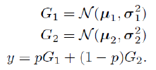
为了理解其工作原理,我们将考虑高斯混合模型最简单的有趣情况:仅包含两个高斯混合的组合。现在的假设是,样本来自那个高斯分布。如果选择高斯分布一的概率是 p,那么整个模型看起来是这样的(其中 N(μ,σ2) 表示均值为 μ、标准差为 σ 的高斯分布):
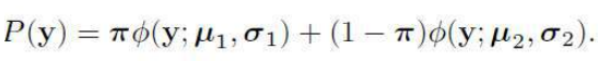
如果 p 的概率分布写成 π,那么概率密度为:
寻找这个问题的最大似然解(实际上是最大对数似然)涉及计算方程在所有训练数据上的对数和,并进行微分,这会相当困难。幸运的是,有一种方法可以绕过它。我们需要掌握的关键洞察是,如果我们知道每个数据点来自两个高斯分量中的哪一个,那么计算就会变得容易。每个分量的均值和标准差可以从属于该分量的数据点中计算出来,这将不成问题。
尽管我们不知道每个数据点来自哪个分量,但我们可以假装知道,通过引入一个新的变量 f。如果 ,则数据来自高斯分布一;如果 ,则数据来自高斯分布二。
这是 EM 算法典型的初始步骤:添加潜在变量。现在我们只需要弄清楚如何对其进行优化。这时,算法被称为“期望-最大化”的原因就变得清晰了。我们对变量 f 了解不多(这不足为奇,因为是我们创造了它),但我们可以从数据中计算它的期望值(即我们“期望”看到的值,也就是平均值):
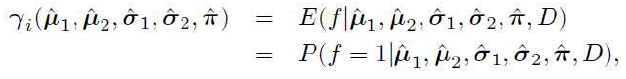
E[f∣x,D]
其中 D 表示数据。注意,由于我们设置了 ,这意味着我们选择高斯分布二。
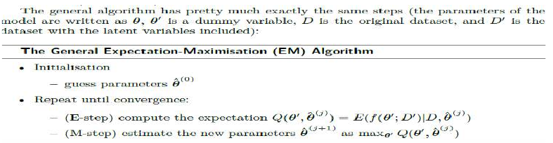
计算这个期望值的过程称为 E-步(Expectation-step)。然后,这个期望值的估计值在模型参数(两个高斯分布的参数和混合参数 π)上进行最大化,这称为 M-步(Maximization-step)。这需要对期望值关于每个模型参数进行微分。这两个步骤简单地迭代,直到算法收敛。请注意,估计值永远不会变小,并且事实证明,EM 算法保证会达到局部最大值。为了了解这对于两分量高斯混合模型是怎样的,我们将更深入地研究该算法:
将 EM 算法应用于问题的诀窍在于识别要包含的正确潜在变量,然后简单地逐步执行这些步骤。它们是用于各种统计学习问题的非常强大的方法。我们现在将把注意力转向更简单的事情,那就是我们如何利用附近数据点的信息来决定分类输出。为此,我们根本不使用数据模型,而是直接使用可用数据。
The basic idea of the EM algorithm is that sometimes it is easier to add extra variables that are
not actually known (called hidden or latent variables) and then to maximise the function over those
variables. This might seem to be making a problem much more complicated than it needs to be, but it
turns out for many problems that it makes finding the solution significantly easier.
In order to see how it works, we will consider the simplest interesting case of the Gaussian
mixture model: a combination of just two Gaussian mixtures. The assumption now is that sample from
that Gaussian. If the probability of picking Gaussian one is p, then the entire model looks like this
(where N(μ, σ2) specifies a Gaussian distribution with mean μ and standard deviation σ):
If the probability distribution of p is written as π, then the probability density is:
Finding the maximum likelihood solution (actually the maximum log likelihood) to this problem
is then a case of computing the sum of the logarithm of Equation over all of the training data, and
differentiating it, which would be rather difficult. Fortunately, there is a way around it. The key insight
that we need is that if we knew which of the two Gaussian components the datapoint came from, then
the computation would be easy. The mean and standard deviation for each component could be
computed from the datapoints that belong to that component, and there would not be a problem.
Although we don’t know which component each datapoint came from, we can pretend we do, by
introducing a new variable f. If f = 0 then the data came from Gaussian one, if f = 1 then it came from
Gaussian two.
This is the typical initial step of an EM algorithm: adding latent variables. Now we just need to
work out how to optimise over them. This is the time when the reason for the algorithm being called
expectation-maximisation becomes clear.We don’t know much about variable f (hardly surprising, since
we invented it), but we can compute its expectation (that is, the value that we ‘expect’ to see, which is
the mean average) from the data:
where D denotes the data. Note that since we have set f = 1 this means that we are choosing GaussiaComputing the value of this expectation is known as the E-step. Then this estimate of the
expectation is maximised over the model parameters (the parameters of the two Gaussians and the
mixing parameter π), the M-step. This requires differentiating the expectation with respect to each of
the model parameters. These two steps are simply iterated until the algorithm converges. Note that the
estimate never gets any smaller, and it turns out that EM algorithms are guaranteed to reach a local
maxima. To see how this looks for the two-component Gaussian mixture, we’ll take a closer look at the
algorithm:
The trick with applying EM algorithms to problems is in identifying the correct latent variables
to include, and then simply working through the steps. They are very powerful methods for a wide
variety of statistical learning problems. We are now going to turn our attention to something much
simpler, which is how we can use information about nearby datapoints to decide on classification
output. For this we don’t use a model of the data at all, but directly use the data that is available.