机器学习
假设你身处一家夜总会,决定跳舞。你不太可能知道正在播放的这首歌的舞步,所以你可能会通过观察身边的人在做什么来尝试弄清楚自己该怎么跳。你可以做的第一件事就是选择离你最近的人,然后模仿他们。然而,由于夜总会里大多数人也不太可能知道所有的舞步,你可能会决定多看几个人,然后模仿他们大多数人的动作。这几乎就是最近邻方法背后的核心思想:如果我们没有一个描述数据的模型,那么最好的办法就是查看相似的数据,并选择与它们属于同一类别。
我们有数据点在输入空间中的位置,所以我们只需要找出训练数据中哪些点与它接近。这需要计算到训练集中每个数据点的距离,这相对来说成本较高:如果我们处于普通的欧几里得空间中,那么我们必须计算 d 次减法和 d 次平方(我们可以忽略平方根,因为我们只想知道哪些点最近,而不是实际距离),而且这必须执行 O(N2) 次。然后我们可以识别出测试点的 k 个最近邻,并将测试点的类别设置为这些最近邻中最常见的类别。
k 的选择并非微不足道。如果 k 太小,最近邻方法对噪声敏感;如果 k 太大,准确性会降低,因为考虑了太远的点。改变 k 的大小对决策边界可能产生的一些影响如下图 5 所示。
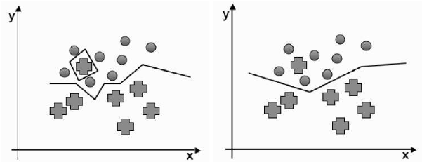
图 5:最近邻决策边界,左侧:一个邻居,右侧:两个邻居。
这种方法受到维度灾难的影响。首先,如上所示,随着维数的增加,计算成本会变高。这并没有乍看起来那么糟糕:有一些方法集,例如 KD-树(将在后续主题中讨论),可以在 O(NlogN) 时间内计算出来。然而,更重要的是,随着维度的增加,与其他数据点的距离往往会增加。此外,它们可能在各种不同的方向上都很远——有些点在某些维度上相对接近,但在其他维度上却很远。有一些方法可以解决这些问题,称为自适应最近邻方法,在章节末尾的“进一步阅读”部分有对它们的引用。
在实现过程中唯一需要注意的部分是,当在最近的点中发现多个类别时该怎么办,但即使如此,实现仍然简单:
# 假设 sorted_distances 是一个包含 (距离, 类别) 对的列表,按距离排序
# 假设 k 是要考虑的邻居数量
# 假设 classes 是所有可能的类别列表

# 统计前 k 个邻居中每个类别的出现次数
class_counts = {}
for i in range(k):
    distance, current_class = sorted_distances[i]
    class_counts[current_class] = class_counts.get(current_class, 0) + 1

# 找到出现次数最多的类别(多数投票)
# 如果有平局,可以根据具体需求选择处理方式(例如,随机选择,或选择距离最近的那个类别)
max_count = 0
most_common_class = None
for current_class, count in class_counts.items():
    if count > max_count:
        max_count = count
        most_common_class = current_class
    # 可以添加处理平局的逻辑,例如:
    # elif count == max_count:
    #     pass # 根据需求决定如何处理平局

# 返回最常见的类别作为预测结果
# return most_common_class
接下来,我们将研究如何将这些方法用于回归,然后我们将探讨如何尽可能高效地执行距离计算的问题,这在上面的代码中虽然简单但效率低下。然后我们将简要考虑欧几里得距离是否总是计算距离最有效的方式,以及存在哪些替代方案。
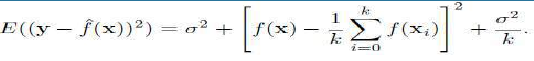
对于 k-最近邻算法,偏差-方差分解可以计算为:
这里的解释是,当 k 很小,只考虑少数邻居时,模型具有灵活性并且可以很好地表示底层模型,但它会犯错误(具有高方差),因为数据相对较少。随着 k 的增加,方差减小,但代价是灵活性降低,从而导致偏差增加。
Suppose that you are in a nightclub and decide to dance. It is unlikely that you will know the
dance moves for the particular song that is playing, so you will probably try to work out what to do by
looking at what the people close to you are doing. The first thing you could do would be just to pick the
person closest to you and copy them. However, since most of the people who are in the nightclub are
also unlikely to know all the moves, you might decide to look at a few more people and do what most of
them are doing. This is pretty much exactly the idea behind nearest neighbour methods: if we don’t
have a model that describes the data, then the best thing to do is to look at similar data and choose to
be in the same class as them.
We have the datapoints positioned within input space, so we just need to work out which of the
training data are close to it. This requires computing the distance to each datapoint in the training set,
which is relatively expensive: if we are in normal Euclidean space, then we have to compute d
subtractions and d squarings (we can ignore the square root since we only want to know which points
are the closest, not the actual distance) and this has to be done O(N2) times. We can then identify the k
nearest neighbours to the test point, and then set the class of the test point to be the most common
one out of those for the nearest neighbours. The choice of k is not trivial. Make it too small and nearest
neighbour methods are sensitive to noise, too large and the accuracy reduces as points that are too far
away are considered. Some possible effects of changing the size of k on the decision boundary are
shown in below Figure 5.
FIGURE 5: The nearest neighbours decision boundary with left: one neighbour and right:
two neighbours.
This method suffers from the curse of dimensionality. First, as shown above, the computational
costs get higher as the number of dimensions grows. This is not as bad as it might appear at first: there
are sets of methods such as KD-Trees (will discuss in upcoming topics) that compute this in O(N log N)
time. However, more importantly, as the number of dimensions increases, so the distance to other
datapoints tends to increase. In addition, they can be far away in a variety of different directions—there
might be points that are relatively close in some dimensions, but a long way in others. There are
methods for dealing with these problems, known as adaptive nearest neighbour methods, and there is a
reference to them in the Further Reading section at the end of the chapter.
The only part of this that requires any care during the implementation is what to do when there
is more than one class found in the closest points, but even with that the implementation is nice and
simple:
77
We are going to look next at how we can use these methods for regression, before we turn to the
question of how to perform the distance calculations as efficiently as possible, something that is done
simply but inefficiently in the code above. We will then consider briefly whether or not the Euclidean
distance is always the most useful way to calculate distances, and what alternatives there are.
For the k-nearest neighbours algorithm the bias-variance decomposition can be computed as:
The way to interpret this is that when k is small, so that there are few neighbours considered, the model
has flexibility and can represent the underlying model well, but that it makes mistakes (has high
variance) because there is relatively little data. As k increases, the variance decreases, but at the cost of
less flexibility and so more bias.