机器学习
如前所述,计算所有点对之间的距离在计算上非常昂贵。幸运的是,与计算机科学中的许多问题一样,设计一个高效的数据结构可以大大减少计算开销。对于寻找最近邻的问题,首选的数据结构是 KD 树。它自 20 世纪 70 年代后期由 Friedman 和 Bentley 设计以来就一直存在,它将寻找最近邻的成本降低到 O(log N)(对于 O(N) 的存储)。树的构建是 O(N log² N),其中大部分计算成本在于中位数的计算,使用朴素算法需要排序,因此是 O(N log N),或者可以使用随机算法在 O(N) 时间内计算。
KD 树背后的思想非常简单。你通过每次选择一个维度进行分割来创建一棵二叉树,并将分割线穿过该维度上点坐标的中位数。这些点本身最终成为树的叶子节点。构建树的过程与构建二叉树的通常步骤大致相同:我们确定一个位置将其分成两个选择,左和右,然后沿着树向下继续。这使得用递归方式编写算法很自然。选择分割什么以及在哪里分割是 KD 树的特殊之处。每一步只分割一个维度,分割的位置通过计算该维度上要分割点中位数来找到,然后将分割线放在那里。通常,选择分割哪个维度会在不同的选择之间交替进行,或者可以随机选择。下面的算法根据树的当前深度循环遍历可能的维度,因此在二维空间中它会交替进行水平和垂直分割。
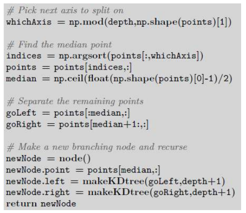
构造方法的核心是一个简单的递归函数,它选择要分割的轴,找到该轴上的中位值,并根据该值分离点,这在 Python 中可以写成:
假设我们有七个二维点要从中构建一棵树:(5, 4), (1, 6), (6, 1), (7, 5), (2, 7), (2, 2), (5, 8)(如图 7 所示)。
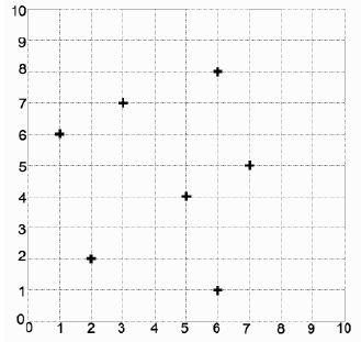
图 7:2D 数据的初始集合。
算法会首先选择第一个坐标进行分割,这里的中位点是 5,所以分割线穿过 。在线左侧的点中,中位 y 坐标是 6,而在线右侧的点中,中位 y 坐标是 5。此时我们已经分离了所有的点,所以算法终止,得到图 8 所示的分割和图 9 所示的树。
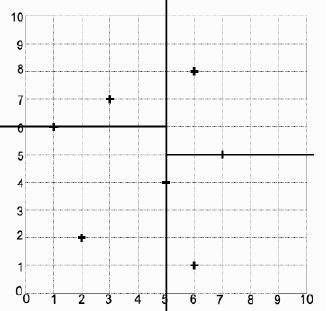
图 8:KD 树找到的分割和叶子点。
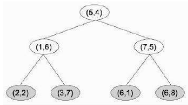
图 9:创建分割的 KD 树。
搜索树与任何其他二叉树相同;我们更感兴趣的是找到测试点的最近邻。这相当容易:从树的根节点开始,你递归地向下遍历树,每次只比较一个维度,直到找到一个包含测试点的区域的叶子节点。使用图 9 所示的树,我们引入测试点 (3, 5),它找到 (2, 2) 作为 (3, 5) 所在框的叶子节点。然而,查看图 10,我们发现这根本不是最近的点,所以我们需要做更多的工作。
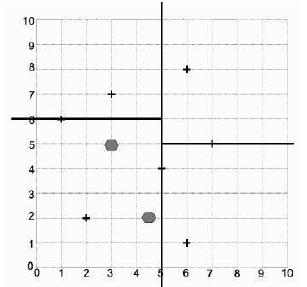
图 10:KD 树示例的两个测试点。
As was mentioned above, computing the distances between all pairs of points is very
computationally expensive. Fortunately, as with many problems in computer science, designing an
efficient data structure can reduce the computational overhead a lot. For the problem of finding
nearest neighbours the data structure of choice is the KD-Tree. It has been around since the late 1970s,
when it was devised by Friedman and Bentley, and it reduces the cost of finding a nearest neighbour to
O(log N) for O(N) storage. The construction of the tree is O(N log2 N), with much of the computational
cost being in the computation of the median, which with a naïve algorithm requires a sort and is
therefore O(N log N), or can be computed with a randomised algorithm in O(N) time.
The idea behind the KD-tree is very simple. You create a binary tree by choosing one dimension
at a time to split into two, and placing the line through the median of the point coordinates of that
dimension. The points themselves end up as leaves of the tree. Making the tree follows pretty much the
same steps as usual for constructing a binary tree: we identify a place to split into two choices, left and
right, and then carry on down the tree. This makes it natural to write the algorithm recursively. The
choice of what to split and where is what makes the KD-tree special. Just one dimension is split in each
step, and the position of the split is found by computing the median of the points that are to be split in
that one dimension, and putting the line there. In general, the choice of which dimension to spalternates through the different choices, or it can be made randomly. The algorithm below cycles
through the possible dimensions based on the depth of the tree so far, so that in two dimensions it
alternates horizontal and vertical splits.
The centre of the construction method is simply a recursive function that picks the axis to split
on, finds the median value on that axis, and separates the points according to that value, which in
Python can be written as:
Suppose that we had seven two-dimensional points to make a tree from: (5, 4), (1, 6), (6, 1), (7, 5), (2,
7), (2, 2), (5, 8) (as plotted in Figure 7).
FIGURE 7: The initial set of 2D data.
The algorithm will pick the first coordinate to split on initially, and the median point here is 5, so the
split is through x = 5. Of those on the left of the line, the median y coordinate is 6, and for those on the
right it is 5. At this point we have separated all the points, and so the algorithm terminates with the split
shown in Figure 8 and the tree shown in Figure 9.
81
FIGURE 8: The splits and leaf points found by the KD-tree.
FIGURE 9: The KD-tree that made the splits.
Searching the tree is the same as any other binary tree; we are more interested in finding the nearest
neighbours of a test point. This is fairly easy: starting at the root of the tree you recurse down through
the tree comparing just one dimension at a time until you find a leaf node that is in the region
containing the test point. Using the tree shown in Figure 9 we introduce the test point (3, 5), which
finds (2, 2) as the leaf for the box that (3, 5) is in. However, looking at Figure 10 we see that this is not
the closest point at all, so we need to do some more work.
FIGURE 10 Two test points for the example KD-tree.