机器学习
- 考虑一个马尔可夫决策过程 (MDP),其中智能体可以感知其环境的一组不同的状态 S,并拥有一组可以执行的动作 A。
- 在每个离散时间步 t,智能体感知当前状态 st,选择并执行一个当前动作 at。
- 环境通过给予智能体一个奖励 并产生后续状态 来响应。这里,函数 δ(st,at) 和 r(st,at) 仅依赖于当前状态和动作,而不依赖于之前的状态或动作。
智能体的任务是学习一个策略 ,用于根据当前观察到的状态 st 来选择其下一个动作 at;即 。
我们应该如何精确地指定我们希望智能体学习哪种策略 π 呢?
-
一种方法是要求策略能够为机器人带来随时间累积的最大可能奖励。
- 为了更精确地阐述这个要求,定义从任意初始状态 st 遵循任意策略 π 所获得的累积价值 Vπ(st) 如下:
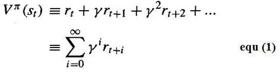
其中,奖励序列 rt+i 是通过从状态 st 开始并反复使用策略 π 选择动作而产生的。
- 这里 是一个常数,它决定了延迟奖励与即时奖励的相对价值。如果我们设置 ,则只考虑即时奖励。当我们设置 γ 更接近 1 时,未来奖励相对于即时奖励会得到更大的重视。
- 数量 Vπ(st) 被称为策略 π 从初始状态 st 获得的折扣累积奖励。对未来奖励相对于即时奖励进行折扣是合理的,因为在许多情况下,我们更喜欢尽早获得奖励。
- 为了更精确地阐述这个要求,定义从任意初始状态 st 遵循任意策略 π 所获得的累积价值 Vπ(st) 如下:
-
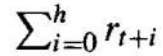
总奖励的其他定义是有限视野奖励(finite horizon reward),它考虑了在有限步数 h 内未折扣的奖励总和。
-
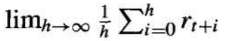
另一种方法是平均奖励(average reward),它考虑了智能体整个生命周期内每时间步的平均奖励。
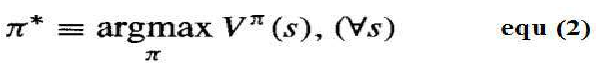
我们要求智能体学习一个最大化所有状态 s 的 Vπ(st) 的策略 π。这样的策略称为最优策略,并用 π∗ 表示。
最优策略的值函数 Vπ∗(s) 记为 V∗(s)。V∗(s) 给出了智能体从状态 s 开始可以获得的最大折扣累积奖励。
示例:
下图描绘了一个简单的网格世界环境:
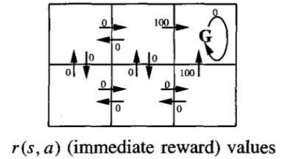
- 图中六个网格方块代表智能体的六种可能的状态或位置。
- 图中的每根箭线代表智能体可以执行的可能动作,以从一个状态移动到另一个状态。
- 与每根箭线关联的数字代表智能体执行相应状态-动作转换时获得的即时奖励 r(s,a)。
- 在这个环境中,除了那些导致进入标记为 G 的状态的转换外,所有状态-动作转换的即时奖励都定义为零。状态 G 作为目标状态,智能体可以通过进入此状态获得奖励。
一旦定义了状态、动作和即时奖励,选择折扣因子 γ 的值,确定最优策略 π∗ 及其值函数 V∗(s)。
让我们选择 。图底部的图表显示了此设置的一种最优策略。
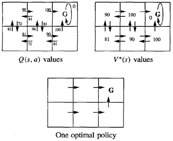
V∗(s) 和 Q(s,a) 的值由 r(s,a) 和折扣因子 得出。图中还显示了对应于最大 Q 值的最优策略。
从底部中心状态获得的折扣未来奖励为:
Consider Markov decision process (MDP) where the agent can perceive a set S of distinct states of
its environment and has a set A of actions that it can perform.
At each discrete time step t, the agent senses the current state st, chooses a current action at, and
performs it.
The environment responds by giving the agent a reward rt = r(st, at) and by producing the
succeeding state st+l = δ(st, at). Here the functions δ(st, at) and r(st, at) depend only on the current
state and action, and not on earlier states or actions.
The task of the agent is to learn a policy, π: S → A, for selecting its next action a, based on the current
observed state st; that is, (st) = at.
How shall we specify precisely which policy π we would like the agent to learn?
1. One approach is to require the policy that produces the greatest possible cumulative reward for the
robot over time.
To state this requirement more precisely, define the cumulative value Vπ (st) achieved by following
an arbitrary policy π from an arbitrary initial state st as follows:
Where, the sequence of rewards rt+i is generated by beginning at state st and by repeatedly using
the policy π to select actions.
Here 0 ≤ γ ≤ 1 is a constant that determines the relative value of delayed versus immediate
rewards. if we set γ = 0, only the immediate reward is considered. As we set γ closer to 1, future
rewards are given greater emphasis relative to the immediate reward.
The quantity Vπ (st) is called the discounted cumulative reward achieved by policy π from initial
state s. It is reasonable to discount future rewards relative to immediate rewards because, in many
cases, we prefer to obtain the reward sooner rather than later.
2. Other definitions of total reward is finite horizon reward,
Considers the undiscounted sum of rewards over a finite number h of steps
3. Another approach is average reward
Considers the average reward per time step over the entire lifetime of the agent.
We require that the agent learn a policy π that maximizes Vπ (st) for all states s. such a policy is called
an optimal policy and denote it by π*
87
Refer the value function Vπ*(s) an optimal policy as V*(s). V*(s) gives the maximum discounted
cumulative reward that the agent can obtain starting from state s.
Example:
A simple grid-world environment is depicted in the diagram
The six grid squares in this diagram represent six possible states, or locations, for the agent.
Each arrow in the diagram represents a possible action the agent can take to move from one state
to another.
The number associated with each arrow represents the immediate reward r(s, a) the agent receives
if it executes the corresponding state-action transition
The immediate reward in this environment is defined to be zero for all state-action transitions
except for those leading into the state labelled G. The state G as the goal state, and the agent can
receive reward by entering this state.
Once the states, actions, and immediate rewards are defined, choose a value for the discount factor γ,
determine the optimal policy π * and its value function V*(s).
Let’s choose γ = 0.9. The diagram at the bottom of the figure shows one optimal policy for this setting.
88
Values of V*(s) and Q(s, a) follow from r(s, a), and the discount factor γ = 0.9. An optimal policy,
corresponding to actions with maximal Q values, is also shown.
The discounted future reward from the bottom centre state is
0+ γ 100+ γ2 0+ γ3 0+... = 90