机器学习
为了更好地理解二项式分布,我们来看下面这个问题:
- 假设我们有一枚磨损变形的硬币,想估计它被抛掷时正面朝上的概率。
- 未知正面朝上的概率 p。我们抛掷硬币 n 次,并记录正面朝上的次数 r。
- 对 p 的估计为 。
- 如果重新进行这个实验,生成一组新的 n 次硬币抛掷,我们可能会发现正面朝上的次数 r 与第一次实验测得的值略有不同,从而得到一个稍有差异的 p 的估计值。
- 二项式分布描述的是:给定 n 次独立抛掷硬币的样本,且硬币正面朝上的真实概率为 p,那么观察到恰好 r 次正面朝上的概率(即 r 从 0 到 n 的每个可能值)是多少。
二项式分布的通用应用场景是:
- 有一个基础实验(例如,抛掷硬币),其结果可以用一个随机变量 Y 来描述。随机变量 Y 可以取两个可能的值(例如, 表示正面朝上, 表示反面朝上)。
- 在基础实验的任何单次试验中, 的概率由某个常数 p 给出,且独立于任何其他实验的结果。因此, 的概率为 。通常情况下,p 是事先未知的,问题在于估计它。
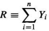
- 进行一系列 n 次独立的基础实验(例如,n 次独立的硬币抛掷),产生序列 Y1,Y2,…,Yn 这组独立的、同分布的随机变量。设 R 表示在这一系列 n 次实验中 的试验次数。
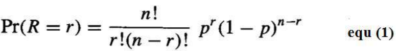
- 随机变量 R 取特定值 r(例如,观察到恰好 r 次正面朝上)的概率由二项式分布给出:
均值、方差和标准差
**均值(期望值)**是随机变量重复抽样所取值的平均值。
定义: 考虑一个随机变量 Y,它取可能的值 y1,…,yn。Y 的期望值(均值),E[Y],是:
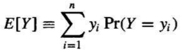
E[Y]=∑i=1nyiP(Y=yi)
方差衡量了随机变量偏离其均值的预期程度。
定义: 随机变量 Y 的方差,Var[Y],是:
![]()
Var[Y]=E[(Y−E[Y])2]
方差描述了使用单次观察 Y 来估计其均值 E[Y] 时预期平方误差。
标准差是方差的平方根,记为 σY。
定义: 随机变量 Y 的标准差,σY,是:
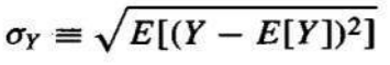
σY=Var[Y]
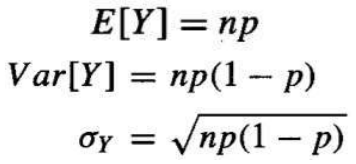
如果随机变量 Y 服从二项式分布,那么其均值、方差和标准差由以下公式给出:
- 均值:
- 方差:
- 标准差:

Consider the following problem for better understanding of Binomial Distribution
Given a worn and bent coin and estimate the probability that the coin will turn up heads when
tossed.
Unknown probability of heads p. Toss the coin n times and record the number of times r that it
turns up heads.
Estimate of p = r / n
If the experiment were rerun, generating a new set of n coin tosses, we might expect the
number of heads r to vary somewhat from the value measured in the first experiment, yielding
a somewhat different estimate for p.
The Binomial distribution describes for each possible value of r (i.e., from 0 to n), the probability
of observing exactly r heads given a sample of n independent tosses of a coin whose true
probability of heads is p.
The general setting to which the Binomial distribution applies is:
1. There is a base experiment (e.g., toss of the coin) whose outcome can be described by a random
variable ‘Y’. The random variable Y can take on two possible values (e.g., Y = 1 if heads, Y = 0 if tails).
2. The probability that Y = 1 on any single trial of the base experiment is given by some constant p,
independent of the outcome of any other experiment. The probability that Y = 0 is therefore (1 - p).
Typically, p is not known in advance, and the problem is to estimate it.
3. A series of n independent trials of the underlying experiment is performed (e.g., n independent coin
tosses), producing the sequence of independent, identically distributed random variables Y1, Y2, . . . ,
Yn. Let R denote the number of trials for which Yi = 1 in this series of n experiments
4. The probability that the random variable R will take on a specific value r (e.g., the probability of
observing exactly r heads) is given by the Binomial distribution
Mean, Variance and Standard Deviation
The Mean (expected value) is the average of the values taken on by repeatedly sampling the random
variable
Definition: Consider a random variable Y that takes on the possible values y1, . . . yn. The expected
value (Mean) of Y, E[Y], is
The Variance captures how far the random variable is expected to vary from its mean value.
Definition: The variance of a random variable Y, Var[Y], is
The variance describes the expected squared error in using a single observation of Y to estimate its
mean E[Y].
The square root of the variance is called the standard deviation of Y, denoted σy
Definition: The standard deviation of a random variable Y, σy, is
In case the random variable Y is governed by a Binomial distribution, then the Mean, Variance and standard
deviation are given by