机器学习
如上所述,遗传算法 (GAS) 采用一种随机束搜索方法来寻找最适应的假设。这种搜索与其他我们在本书中考虑的学习方法截然不同。例如,将遗传算法的假设空间搜索与神经网络反向传播 (BACKPROPAGATION) 的搜索进行对比,反向传播中的梯度下降搜索平稳地从一个假设移动到与其非常相似的新假设。相比之下,遗传算法的搜索可以更加突然,用可能与父代截然不同的子代取代父代假设。请注意,因此遗传算法搜索不太可能陷入困扰梯度下降方法的局部最小值。
在一些遗传算法应用中,一个实际的困难是拥挤问题。拥挤是一种现象,其中种群中某个比其他个体适应度更高的个体迅速繁殖,导致该个体及其非常相似的个体的副本占据了种群的很大一部分。拥挤的负面影响是它降低了种群的多样性,从而减缓了遗传算法的进一步进展。人们已经探索了几种减少拥挤的策略。一种方法是改变选择函数,使用锦标赛选择或排名选择代替适应度比例轮盘赌选择。一个相关的策略是“适应度共享”,其中个体的测量适应度会因种群中存在其他相似个体而降低。第三种方法是限制允许重组形成后代的个体类型。例如,通过只允许最相似的个体重组,我们可以鼓励形成相似个体的簇,或者在种群中形成多个“亚种”。一个相关的方法是在空间上分布个体,并且只允许附近的个体重组。这些技术中有许多都受到生物进化类比的启发。
种群进化与模式定理
有趣的是,我们是否可以数学地描述遗传算法中种群随时间的演化。模式定理 (schema theorem) 提供了一种这样的表征。它基于模式 (schemas) 的概念,即描述位串集合的模式。精确地说,模式是由 0、1 和 * 组成的任何字符串。每个模式代表包含指定 0 和 1 的位串集合,其中每个“”被解释为“不关心”。例如,模式 **010** 代表包含 0010 和 0110 的位串集合。
一个单独的位串可以被视为它所匹配的每个不同模式的代表。例如,位串 0010 可以被认为是 2^4 个不同模式的代表,包括 00**, 0*10,**** 等。类似地,位串种群可以根据它所代表的模式集合以及与每个模式关联的个体数量来理解。
模式定理根据代表每个模式的实例数量来表征遗传算法中种群的演化。令 m(s,t) 表示在时间 t(即第 t 代)种群中模式 s 的实例数量。模式定理根据 m(s,t) 以及模式、种群和遗传算法参数的其他属性来描述 的期望值。
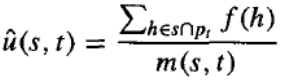
遗传算法中种群的演化取决于选择步骤、重组步骤和变异步骤。让我们首先只考虑选择步骤的影响。令 f(h) 表示个体位串 h 的适应度,fˉ(t) 表示在时间 t 种群中所有个体的平均适应度。令 N 为种群中的个体总数。令 表示个体 h 既是模式 s 的代表,又是时间 t 种群的成员。最后,令 u^(s,t) 表示时间 t 种群中模式 s 实例的平均适应度。
我们有兴趣计算 的期望值,我们将其表示为 。我们可以使用方程中给出的选择概率分布来计算 ,用我们当前的术语可以重新表述如下:
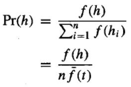
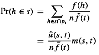
如果我们根据这个概率分布为新种群选择一个成员,那么我们将选择模式 s 的代表的概率是:
上述第二步是根据定义得出的。
方程给出了遗传算法选择单个假设成为模式 s 实例的概率。因此,由创建整个新一代的 N 个独立选择步骤所产生的 s 实例的期望数量,就是 N 乘以这个概率。
方程表明,在第 代模式 s 实例的期望数量与该模式在时间 t 实例的平均适应度 u^(s,t) 成正比,并与时间 t 种群中所有成员的平均适应度 fˉ(t) 成反比。因此,我们可以预期具有高于平均适应度的模式在后续世代中将以越来越高的频率被表示。如果我们将遗传算法视为同时在个体空间中执行其显式并行搜索的同时,也在可能模式空间中执行虚拟并行搜索,那么方程表明更适应的模式将随着时间的推移而增强影响力。
虽然上述分析只考虑了遗传算法的选择步骤,但交叉和变异步骤也必须考虑在内。模式定理只考虑了这些遗传操作符可能的负面影响(例如,随机变异可能会减少 s 的代表数量,与 u^(s,t) 无关),并且只考虑了单点交叉的情况。因此,完整的模式定理提供了模式 s 预期频率的下限,如下所示:
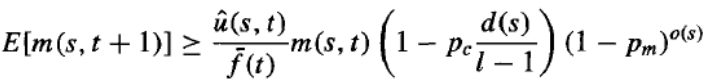
这里,pc 是单点交叉操作符应用于任意个体的概率,pm 是任意个体中任意位被变异操作符变异的概率。o(s) 是模式 s 中定义位的数量,其中 0 和 1 是定义位,但 * 不是。d(s) 是 s 中最左侧和最右侧定义位之间的距离。最后,l 是种群中个体位串的长度。注意,方程中最左侧的项与方程中的项相同,描述了选择步骤的影响。中间项描述了单点交叉操作符的影响——特别是,它描述了表示 s 的任意个体在应用此交叉操作符后仍将表示 s 的概率。最右侧的项描述了表示模式 s 的任意个体在应用变异操作符后仍将表示模式 s 的概率。请注意,单点交叉和变异的影响随着模式中定义位 o(s) 的数量以及定义位之间距离 d(s) 的增加而增加。因此,模式定理可以粗略地解释为:更适应的模式将倾向于增强影响力,特别是包含少量定义位(即包含大量 * 的)的模式,并且特别是在这些定义位在位串中彼此靠近时。模式定理也许是遗传算法中种群演化最广为引用的表征。它不完整的一个方面是未能考虑交叉和变异的( presumably)积极影响。已经提出了许多更新的理论分析,包括基于马尔可夫链模型和统计力学模型的分析。
5.4 Hypothesis Space Search
As illustrated above, GAS employ a randomized beam search method to seek a maximally fit hypothesis.
This search is quite different from that of other learning methods we have considered in this book. To
contrast the hypothesis space search of GAS with that of neural network BACKPROPAGATION, for
example, the radiant descent search in BACKPROPAGATION moves smoothly from one hypothesis to a
new hypothesis that is very similar. In contrast, the GA search can move much more abruptly, replacing
a parent hypothesis by an offspring that may be radically different from the parent. Note the GA search
is therefore less likely to fall into the same kind of local minima that can plague gradient descent
methods.
One practical difficulty in some GA applications is the problem of crowding. Crowding is a phenomenon
in which some individual that is more highly fit than others in the population quickly reproduces, so that
copies of this individual and very similar individuals take over a large fraction of the population. The
negative impact of crowding is that it reduces the diversity of the population, thereby slowing further
progress by the GA. Several strategies have been explored for reducing crowding. One approach is to
alter the selection function, using criteria such as tournament selection or rank selection in place of
fitness proportionate roulette wheel selection. A related strategy is "fitness sharing," in which the
measured fitness of an individual is reduced by the presence of other, similar individuals in the
population. A third approach is to restrict the kinds of individuals allowed to recombine to form
offspring. For example, by allowing only the most similar individuals to recombine, we can encouragthe formation of clusters of similar individuals, or multiple "subspecies" within the population. A related
approach is to spatially distribute individuals and allow only nearby individuals to recombine. Many of
these techniques are inspired by the analogy to biological evolution.
Population Evolution and the Schema Theorem
It is interesting to ask whether one can mathematically characterize the evolution over time of the
population within a GA. The schema theorem provides one such characterization. It is based on the
concept of schemas, or patterns that describe sets of bit strings. To be precise, a schema is any string
composed of 0s, 1s, and *'s. Each schema represents the set of bit strings containing the indicated 0s
and 1s, with each “*” interpreted as a "don't care." For example, the schema 0*10 represents the set of
bit strings that includes exactly 0010 and 01 10.
An individual bit string can be viewed as a representative of each of the different schemas that it
matches. For example, the bit string 0010 can be thought of as a representative of 24 distinct schemas
including 00**, 0* 10, ****, etc. Similarly, a population of bit strings can be viewed in terms of the set
of schemas that it represents and the number of individuals associated with each of these schema.
The schema theorem characterizes the evolution of the population within a GA in terms of the number
of instances representing each schema. Let m(s, t) denote the number of instances of schema s in the
population at time t (i.e., during the tth generation). The schema theorem describes the expected value
of m(s,t+1) in terms of m(s, t) and other properties of the schema, population, and GA algorithm
parameters.
The evolution of the population in the GA depends on the selection step, the recombination step, and
the mutation step. Let us start by considering just the effect of the selection step. Let f denote the
fitness of the individual bit string h and
f t denote the average fitness of all individuals in the
population at time t. Let n be the total number of individuals in the population. Let hs
p , indicate
t
that the individual h is both a representative of schema s and a member of the population at time t.
Finally, let u
s, t denote the average fitness of instances of schema s in the population at time t.
We are interested in calculating the expected value of m(s,t+1), which we denote E[m(s,t+1)]. We can
calculate E[m(s,t+1)] using the probability distribution for selection given in Equation, which can be
restated using our current terminology as follows
Now if we select one member for the new population according to this probability distribution, then the
probability that we will select a representative of schema s is
108
The second step above follows from the fact that by definition,
Equation gives the probability that a single hypothesis selected by the GA will be an instance of schema
s. Therefore, the expected number of instances of s resulting from the n independent selection steps
that create the entire new generation is just n times this probability.
Equation states that the expected number of instances of schema s at generation t+1 is proportional to
the average fitness u
s , t of instances of this schema at time t , and inversely proportional to the
average fitness
f t of all members of the population at time t. Thus, we can expect schemas with
above average fitness to be represented with increasing frequency on successive generations. If we
view the GA as performing a virtual parallel search through the space of possible schemas at the same
time it performs its explicit parallel search through the space of individuals, then Equation indicates that
more fit schemas will grow in influence over time.
While the above analysis considered only the selection step of the GA, the crossover and mutation
steps must be considered as well. The schema theorem considers only the possible negative influence
of these genetic operators (e.g., random mutation may decrease the number of representatives of s,
independent of u
s, t and considers only the case of single-point crossover. The full schema theorem
thus provides a lower bound on the expected frequency of schema s, as follows:
Here, p c is the probability that the single-point crossover operator will be applied
to an arbitrary individual, and pm, is the probability that an arbitrary bit of an arbitrary individual will be
mutated by the mutation operator. o(s) is the number of defined bits in schema s, where 0 and 1 are
defined bits, but * is not. d(s) is the distance between the leftmost and rightmost defined bits in s.
Finally, l is the length of the individual bit strings in the population. Notice the leftmost term in Equation
is identical to the term from Equation and describes the effect of the selection step. The middle term
describes the effect of the single-point crossover operator-in particular, it describes the probability that
an arbitrary individual representing s will still represent s following application of this crossover
operator. The rightmost term describes the probability that an arbitrary individual representing schema
s will still represent schema s following application of the mutation operator. Note that the effects of
single-point crossover and mutation increase with the number of defined bits o(s) in the schema and
with the distance d(s) between the defined bits. Thus, the schema theorem can be roughly interpreted
as stating that more fit schemas will tend to grow in influence, especially schemas containing a small
number of defined bits (i.e., containing a large number of *'s), and especially when these defined bits
109
are near one another within the bit string. The schema theorem is perhaps the most widely cited
characterization of population evolution within a GA. One way in which it is incomplete is that it fails to
consider the (presumably) positive effects of crossover and mutation. Numerous more recent
theoretical analyses have been proposed, including analyses based on Markov chain models and on
statistical mechanics models.