Python机器学习项目
本教程中我们将使用的数据集是威斯康星乳腺癌诊断数据库。该数据集包含乳腺癌肿瘤的各种信息,以及恶性或良性的分类标签。数据集有 569 个实例,即关于 569 个肿瘤的数据,并包含 30 个属性(或特征)的信息,例如肿瘤的半径、纹理、平滑度和面积。
利用这个数据集,我们将构建一个机器学习模型,使用肿瘤信息来预测肿瘤是恶性还是良性。
Scikit-learn 内置了各种数据集,我们可以将其加载到 Python 中,我们想要的数据集也包含在内。导入并加载数据集:
ML Tutorial
...
from sklearn.datasets import load_breast_cancer
# Load dataset
data = load_breast_cancer()
data 变量代表一个像字典一样的 Python 对象。需要考虑的重要字典键是分类标签名称 (target_names)、实际标签 (target)、属性/特征名称 (feature_names) 和属性 (data)。
属性是任何分类器的关键部分。属性捕捉了数据性质的重要特征。考虑到我们试图预测的标签(恶性肿瘤与良性肿瘤),可能有用的属性包括肿瘤的大小、半径和纹理。
为每个重要的信息集创建新变量并分配数据:
ML Tutorial
...
# Organize our data
label_names = data['target_names']
labels = data['target']
feature_names = data['feature_names']
features = data['data']
我们现在为每个信息集都有了列表。为了更好地理解我们的数据集,让我们通过打印类标签、第一个数据实例的标签、特征名称和第一个数据实例的特征值来查看我们的数据:
ML Tutorial
...
# Look at our data
print(label_names)
print(labels[0])
print(feature_names[0])
print(features[0])
如果你运行代码,你将看到以下结果:
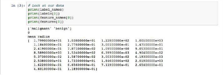
Jupyter Notebook,包含三个 Python 单元格,打印数据集中的第一个实例
如图所示,我们的类名是恶性 (malignant) 和良性 (benign),它们被映射到二进制值 0 和 1,其中 0 代表恶性肿瘤,1 代表良性肿瘤。因此,我们的第一个数据实例是一个恶性肿瘤,其平均半径为 1.79900000e+01。
现在我们已经加载了数据,我们可以处理数据来构建我们的机器学习分类器了。
Step 2 — Importing Scikit-learn’s Dataset
The dataset we will be working with in this tutorial is the Breast Cancer
Wisconsin Diagnostic Database. The dataset includes various information
about breast cancer tumors, as well as classification labels of malignant or
benign. The dataset has 5 6 9 instances, or data, on 569 tumors and
includes information on 30 attributes, or features, such as the radius of
the tumor, texture, smoothness, and area.
Using this dataset, we will build a machine learning model to use
tumor information to predict whether or not a tumor is malignant or
benign.
Scikit-learn comes installed with various datasets which we can load
into Python, and the dataset we want is included. Import and load the
dataset:
ML Tutorial
...
from sklearn.datasets import load_breast_cancer
# Load dataset
data = load_breast_cancer()
T h e data variable represents a Python object that works like a
dictionary. The important dictionary keys to consider are the
classification label names (target_names), the actual labels (target),
the
attribute/feature
names (feature_names), and the attributes
(data).
Attributes are a critical part of any classifier. Attributes capture
important characteristics about the nature of the data. Given the label we
are trying to predict (malignant versus benign tumor), possible useful
attributes include the size, radius, and texture of the tumor.
Create new variables for each important set of information and assign
the data:
ML Tutorial
...
# Organize our data
label_names = data['target_names']
labels = data['target']
feature_names = data['feature_names']
features = data['data']
We now have lists for each set of information. To get a better
understanding of our dataset, let’s take a look at our data by printing our
class labels, the first data instance’s label, our feature names, and the
feature values for the first data instance:
ML Tutorial
...
# Look at our data
print(label_names)
print(labels[0])
print(feature_names[0])
print(features[0])
You’ll see the following results if you run the code:
Alt Jupyter Notebook with three Python cells, which prints the first instance in our dataset
As the image shows, our class names are malignant and benign, which
are then mapped to binary values of 0 and 1, where 0 represents
malignant tumors and 1 represents benign tumors. Therefore, our first
data
instance
is
a
malignant
tumor
whose mean
radius
is
1.79900000e+01.
Now that we have our data loaded, we can work with our data to
build our machine learning classifier.