Python机器学习项目

...
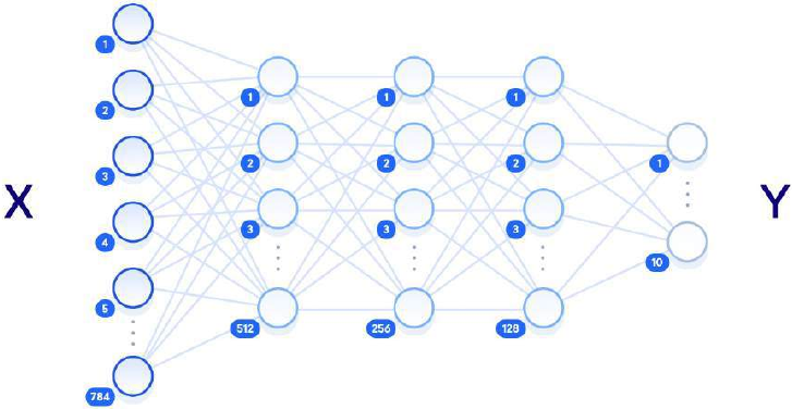
n_input = 784       # 输入层 (28x28 像素)
n_hidden1 = 512     # 第 1 个隐藏层
n_hidden2 = 256     # 第 2 个隐藏层
n_hidden3 = 128     # 第 3 个隐藏层
n_output = 10       # 输出层 (0-9 数字)

...
learning_rate = 1e-4
n_iterations = 1000
batch_size = 128
dropout = 0.5

Step 3 — Defining the Neural Network Architecture
The architecture of the neural network refers to elements such as the
number of layers in the network, the number of units in each layer, and
how the units are connected between layers. As neural networks are
loosely inspired by the workings of the human brain, here the term unit
is used to represent what we would biologically think of as a neuron.
Like neurons passing signals around the brain, units take some values
from previous units as input, perform a computation, and then pass on
the new value as output to other units. These units are layered to form
the network, starting at a minimum with one layer for inputting values,
and one layer to output values. The term hidden layer is used for all of
the layers in between the input and output layers, i.e. those “hidden”
from the real world.
Different architectures can yield dramatically different results, as the
performance can be thought of as a function of the architecture among
other things, such as the parameters, the data, and the duration of
training.
Add the following lines of code to your file to store the number of
units per layer in global variables. This allows us to alter the network
architecture in one place, and at the end of the tutorial you can test for
yourself how different numbers of layers and units will impact the
results of our model:
main.py
...
n_input = 784
 # input layer (28x28 pixels)
n_hidden1 = 512
 # 1st hidden layer
n_hidden2 = 256
 # 2nd hidden layer
n_hidden3 = 128
 # 3rd hidden layer
n_output = 10
 # output layer (0-9 digits)
The following diagram shows a visualization of the architecture we’ve
designed, with each layer fully connected to the surrounding layers:
Diagram of a neural network
The term “deep neural network” relates to the number of hidden
layers, with “shallow” usually meaning just one hidden layer, and
“deep” referring to multiple hidden layers. Given enough training data, a
shallow neural network with a sufficient number of units should
theoretically be able to represent any function that a deep neural network
can. But it is often more computationally efficient to use a smaller deep
neural network to achieve the same task that would require a shallow
network with exponentially more hidden units. Shallow neural networks
also
 often
 encounter
 overfitting,
 where
 the network essentially
memorizes the training data that it has seen, and is not able to generalize
the knowledge to new data. This is why deep neural networks are more
commonly used: the multiple layers between the raw input data and the
output label allow the network to learn features at various levels of
abstraction, making the network itself better able to generalize.
Other elements of the neural network that need to be defined here are
the hyperparameters. Unlike the parameters that will get updated during
training, these values are set initially and remain constant throughout the
process. In your file, set the following variables and values:
main.py
...
learning_rate = 1e-4
n_iterations = 1000
batch_size = 128
dropout = 0.5
The learning rate represents how much the parameters will adjust at
each step of the learning process. These adjustments are a key component
of training: after each pass through the network we tune the weights
slightly to try and reduce the loss. Larger learning rates can converge
faster, but also have the potential to overshoot the optimal values as they
are updated. The number of iterations refers to how many times we go
through the training step, and the batch size refers to how many training
examples we are using at each step. The dropout variable represents a
threshold at which we eliminate some units at random. We will be using
dropout in our final hidden layer to give each unit a 50% chance of
being eliminated at every training step. This helps prevent overfitting.
We have now defined the architecture of our neural network, and the
hyperparameters that impact the learning process. The next step is to
build the network as a TensorFlow graph.