Python机器学习项目

在强化学习中，神经网络有效地根据状态和动作输入预测 Q 值，并使用表格存储所有可能的值，但这在复杂的游戏中变得不稳定。深度强化学习 (Deep Reinforcement Learning) 转而使用神经网络来近似 Q-函数。有关更多详细信息，请参阅 理解深度 Q-学习。

为了让你熟悉在步骤 1 中安装的深度学习库 TensorFlow，你将使用 TensorFlow 的抽象重新实现迄今为止使用的所有逻辑，并且你将使用神经网络来近似你的 Q-函数。然而，你的神经网络将极其简单：你的输出 Q(s) 是一个矩阵 W 乘以你的输入 s。这被称为带有一个全连接层的神经网络：

Q(s)=Ws

重申一下，目标是使用 TensorFlow 的抽象重新实现我们已经构建的机器人中的所有逻辑。这将使你的操作更高效，因为 TensorFlow 可以在 GPU 上执行所有计算。

首先，复制你步骤 3 中的 Q-表脚本：

cp bot_3_q_table.py bot_4_q_network.py

然后使用 nano 或你喜欢的文本编辑器打开新文件：

nano bot_4_q_network.py

首先，更新文件顶部的注释：

/AtariBot/bot_4_q_network.py

"""
Bot 4 -- Use Q-learning network to train bot
"""
. . .

接下来，通过在 import random 下方添加 import tensorflow as tf 导入 TensorFlow 包。此外，在 np.random.seed(0) 正下方添加 tf.set_random_seed(0)。这将确保此脚本的结果在所有会话中都是可重复的：

/AtariBot/bot_4_q_network.py

. . .
import random
import tensorflow as tf # 新增
random.seed(0)
np.random.seed(0)
tf.set_random_seed(0) # 新增
. . .

在文件顶部重新定义你的超参数以匹配以下内容，并添加一个名为 exploration_probability 的函数，它将返回每一步的探索概率。请记住，在这种情况下，“探索”意味着采取随机行动，而不是采取 Q 值估计推荐的行动：

/AtariBot/bot_4_q_network.py

. . .
num_episodes = 4000
discount_factor = 0.99
learning_rate = 0.15
report_interval = 500
exploration_probability = lambda episode: 50. / (episode + 10) # 新增
report = '100-ep Average: %.2f . Best 100-ep Average: %.2f . Average: ' \
         '%.2f (Episode %d)'
. . .

接下来，你将添加一个独热编码 (one-hot encoding) 函数。简而言之，独热编码是将变量转换为有助于机器学习算法做出更好预测的形式的过程。如果你想了解更多关于独热编码的信息，可以查看 计算机视觉中的对抗性示例：如何构建和欺骗基于情感的狗过滤器。

在 report = ... 正下方，添加一个 one_hot 函数：

/AtariBot/bot_4_q_network.py

. . .
report = '100-ep Average: %.2f . Best 100-ep Average: %.2f . Average: ' \
         '%.2f (Episode %d)'

def one_hot(i: int, n: int) -> np.array: # 新增
    """Implements one-hot encoding by selecting the ith standard basis
    vector"""
    return np.identity(n)[i].reshape((1, -1))

def print_report(rewards: List, episode: int):
. . .

接下来，你将使用 TensorFlow 的抽象重写你的算法逻辑。但在那之前，你需要首先为你的数据创建占位符。

在你的 main 函数中，在 rewards=[] 正下方，插入以下高亮内容。在这里，你为时间 t（作为 obs_t_ph）和时间 t+1（作为 obs_tp1_ph）的观察定义了占位符，以及你的动作、奖励和 Q 目标（作为 q_target_ph）的占位符：

/AtariBot/bot_4_q_network.py

. . .
def main():
    env = gym.make('FrozenLake-v0') # create the game
    env.seed(0) # make results reproducible
    rewards = []
    # 1. Setup placeholders # 新增以下内容
    n_obs, n_actions = env.observation_space.n, env.action_space.n
    obs_t_ph = tf.placeholder(shape=[1, n_obs], dtype=tf.float32)
    obs_tp1_ph = tf.placeholder(shape=[1, n_obs], dtype=tf.float32)
    act_ph = tf.placeholder(tf.int32, shape=())
    rew_ph = tf.placeholder(shape=(), dtype=tf.float32)
    q_target_ph = tf.placeholder(shape=[1, n_actions], dtype=tf.float32)
    Q = np.zeros((env.observation_space.n, env.action_space.n)) # 原有行
    for episode in range(1, num_episodes + 1):
. . .

在以 q_target_ph = 开始的行正下方，插入以下高亮行。此代码通过计算所有 a 的 Q(s,a) 来创建 q_current，并计算所有 a′ 的 Q(s′,a′) 来创建 q_target，从而开始你的计算：

/AtariBot/bot_4_q_network.py

. . .
rew_ph = tf.placeholder(shape=(), dtype=tf.float32)
q_target_ph = tf.placeholder(shape=[1, n_actions], dtype=tf.float32)
# 2. Setup computation graph # 新增以下内容
W = tf.Variable(tf.random_uniform([n_obs, n_actions], 0, 0.01))
q_current = tf.matmul(obs_t_ph, W)
q_target = tf.matmul(obs_tp1_ph, W)
Q = np.zeros((env.observation_space.n, env.action_space.n)) # 原有行
for episode in range(1, num_episodes + 1):
. . .

再次在你添加的最后一行正下方，插入以下高亮代码。前两行等同于步骤 3 中计算 Qtarget 的行，其中 Qtarget = reward + discount_factor * np.max(Q[state2, :])。接下来的两行设置你的损失，而最后一行计算最大化你的 Q 值的动作：

/AtariBot/bot_4_q_network.py

. . .
q_current = tf.matmul(obs_t_ph, W)
q_target = tf.matmul(obs_tp1_ph, W)
q_target_max = tf.reduce_max(q_target_ph, axis=1) # 新增
q_target_sa = rew_ph + discount_factor * q_target_max # 新增
q_current_sa = q_current[0, act_ph] # 新增
error = tf.reduce_sum(tf.square(q_target_sa - q_current_sa)) # 新增
pred_act_ph = tf.argmax(q_current, 1) # 新增
Q = np.zeros((env.observation_space.n, env.action_space.n)) # 原有行
for episode in range(1, num_episodes + 1):
. . .

设置好算法和损失函数后，定义你的优化器：

/AtariBot/bot_4_q_network.py

. . .
error = tf.reduce_sum(tf.square(q_target_sa - q_current_sa))
pred_act_ph = tf.argmax(q_current, 1)
# 3. Setup optimization # 新增以下内容
trainer = tf.train.GradientDescentOptimizer(learning_rate=learning_rate)
update_model = trainer.minimize(error)
Q = np.zeros((env.observation_space.n, env.action_space.n)) # 原有行
for episode in range(1, num_episodes + 1):
. . .

接下来，设置游戏循环的主体。为此，将数据传递给 TensorFlow 占位符，TensorFlow 的抽象将处理 GPU 上的计算，返回算法的结果。

首先删除旧的 Q-表和逻辑。具体来说，删除定义 Q（在 for 循环之前）、noise（在 while 循环中）、action、Qtarget 和 Q[state, action] 的行。将 state 重命名为 obs_t，将 state2 重命名为 obs_tp1，以与你之前设置的 TensorFlow 占位符对齐。完成后，你的 for 循环将与以下内容匹配：

/AtariBot/bot_4_q_network.py

. . .
# 3. Setup optimization
trainer = tf.train.GradientDescentOptimizer(learning_rate=learning_rate)
update_model = trainer.minimize(error)
for episode in range(1, num_episodes + 1): # 调整缩进
    obs_t = env.reset() # 更改变量名
    episode_reward = 0
    while True:
        obs_tp1, reward, done, _ = env.step(action) # 更改变量名
        episode_reward += reward
        obs_t = obs_tp1 # 更改变量名
        if done:
            ...

在 for 循环上方，添加以下两行高亮代码。这些行初始化一个 TensorFlow 会话，该会话反过来管理在 GPU 上运行操作所需的资源。第二行初始化计算图中的所有变量；例如，在更新权重之前将其初始化为 0。此外，你将把 for 循环嵌套在 with 语句中，因此将整个 for 循环缩进四个空格：

/AtariBot/bot_4_q_network.py

. . .
trainer = tf.train.GradientDescentOptimizer(learning_rate=learning_rate)
update_model = trainer.minimize(error)

with tf.Session() as session: # 新增
    session.run(tf.global_variables_initializer()) # 新增
    for episode in range(1, num_episodes + 1): # 调整缩进
        obs_t = env.reset()
        ...

在 obs_tp1, reward, done, _ = env.step(action) 行之前，插入以下行来计算动作。此代码评估相应的占位符，并以一定概率用随机动作替换动作：

/AtariBot/bot_4_q_network.py

. . .
    while True:
        # 4. Take step using best action or random action # 新增以下内容
        obs_t_oh = one_hot(obs_t, n_obs)
        action = session.run(pred_act_ph, feed_dict={obs_t_ph: obs_t_oh})[0]
        if np.random.rand(1) < exploration_probability(episode):
            action = env.action_space.sample()
. . .

在包含 env.step(action) 的行之后，插入以下内容以训练神经网络来估计你的 Q 值函数：

/AtariBot/bot_4_q_network.py

. . .
        obs_tp1, reward, done, _ = env.step(action)
        # 5. Train model # 新增以下内容
        obs_tp1_oh = one_hot(obs_tp1, n_obs)
        q_target_val = session.run(q_target, feed_dict={
            obs_tp1_ph: obs_tp1_oh
        })
        session.run(update_model, feed_dict={
            obs_t_ph: obs_t_oh,
            rew_ph: reward,
            q_target_ph: q_target_val,
            act_ph: action
        })
        episode_reward += reward
. . .

你的最终文件将与此源代码匹配：

/AtariBot/bot_4_q_network.py

"""
Bot 4 -- Use Q-learning network to train bot
"""
from typing import List
import gym
import numpy as np
import random
import tensorflow as tf

random.seed(0)
np.random.seed(0)
tf.set_random_seed(0)

num_episodes = 4000
discount_factor = 0.99
learning_rate = 0.15
report_interval = 500
exploration_probability = lambda episode: 50. / (episode + 10)
report = '100-ep Average: %.2f . Best 100-ep Average: %.2f . Average: ' \
         '%.2f (Episode %d)'

def one_hot(i: int, n: int) -> np.array:
    """Implements one-hot encoding by selecting the ith standard basis
    vector"""
    return np.identity(n)[i].reshape((1, -1))

def print_report(rewards: List, episode: int):
    """Print rewards report for current episode
    - Average for last 100 episodes
    - Best 100-episode average across all time
    - Average for all episodes across time
    """
    print(report % (
        np.mean(rewards[-100:]),
        max([np.mean(rewards[i:i+100]) for i in range(len(rewards) - 100)]),
        np.mean(rewards),
        episode))

def main():
    env = gym.make('FrozenLake-v0')  # create the game
    env.seed(0)  # make results reproducible
    rewards = []

    # 1. Setup placeholders
    n_obs, n_actions = env.observation_space.n, env.action_space.n
    obs_t_ph = tf.placeholder(shape=[1, n_obs], dtype=tf.float32)
    obs_tp1_ph = tf.placeholder(shape=[1, n_obs], dtype=tf.float32)
    act_ph = tf.placeholder(tf.int32, shape=())
    rew_ph = tf.placeholder(shape=(), dtype=tf.float32)
    q_target_ph = tf.placeholder(shape=[1, n_actions], dtype=tf.float32)

    # 2. Setup computation graph
    W = tf.Variable(tf.random_uniform([n_obs, n_actions], 0, 0.01))
    q_current = tf.matmul(obs_t_ph, W)
    q_target = tf.matmul(obs_tp1_ph, W)

    q_target_max = tf.reduce_max(q_target_ph, axis=1)
    q_target_sa = rew_ph + discount_factor * q_target_max
    q_current_sa = q_current[0, act_ph]

    error = tf.reduce_sum(tf.square(q_target_sa - q_current_sa))
    pred_act_ph = tf.argmax(q_current, 1)

    # 3. Setup optimization
    trainer = tf.train.GradientDescentOptimizer(learning_rate=learning_rate)
    update_model = trainer.minimize(error)

    with tf.Session() as session:
        session.run(tf.global_variables_initializer())

        for episode in range(1, num_episodes + 1):
            obs_t = env.reset()
            episode_reward = 0
            while True:
                # 4. Take step using best action or random action
                obs_t_oh = one_hot(obs_t, n_obs)
                action = session.run(pred_act_ph, feed_dict={obs_t_ph: obs_t_oh})[0]
                if np.random.rand(1) < exploration_probability(episode):
                    action = env.action_space.sample()

                obs_tp1, reward, done, _ = env.step(action)

                # 5. Train model
                obs_tp1_oh = one_hot(obs_tp1, n_obs)
                q_target_val = session.run(q_target, feed_dict={
                    obs_tp1_ph: obs_tp1_oh
                })
                session.run(update_model, feed_dict={
                    obs_t_ph: obs_t_oh,
                    rew_ph: reward,
                    q_target_ph: q_target_val,
                    act_ph: action
                })

                episode_reward += reward
                obs_t = obs_tp1

                if done:
                    rewards.append(episode_reward)
                    if episode % report_interval == 0:
                        print_report(rewards, episode)
                    break
        print_report(rewards, -1)

if __name__ == '__main__':
    main()

保存文件，退出编辑器，然后运行脚本：

python bot_4_q_network.py

你的输出将精确地以以下内容结束：

Output
100-ep Average: 0.11 . Best 100-ep Average: 0.11 . Average: 0.05 (Episode 500)
100-ep Average: 0.41 . Best 100-ep Average: 0.54 . Average: 0.19 (Episode 1000)
100-ep Average: 0.56 . Best 100-ep Average: 0.73 . Average: 0.31 (Episode 1500)
100-ep Average: 0.57 . Best 100-ep Average: 0.73 . Average: 0.36 (Episode 2000)
100-ep Average: 0.65 . Best 100-ep Average: 0.73 . Average: 0.41 (Episode 2500)
100-ep Average: 0.65 . Best 100-ep Average: 0.73 . Average: 0.43 (Episode 3000)
100-ep Average: 0.69 . Best 100-ep Average: 0.73 . Average: 0.46 (Episode 3500)
100-ep Average: 0.77 . Best 100-ep Average: 0.79 . Average: 0.48 (Episode 4000)
100-ep Average: 0.77 . Best 100-ep Average: 0.79 . Average: 0.48 (Episode -1)

你现在已经训练了你的第一个深度 Q-学习智能体。对于像《冰冻湖》这样简单的游戏，你的深度 Q-学习智能体需要 4000 个回合进行训练。想象一下如果游戏更复杂，那将需要多少训练样本？事实证明，智能体可能需要数百万个样本。所需的样本数量被称为样本复杂度 (sample complexity)，这个概念将在下一节中进一步探讨。

理解偏差-方差权衡

总的来说，样本复杂度 (sample complexity) 与机器学习中的模型复杂度 (model complexity) 是对立的：

1. 模型复杂度：人们希望有一个足够复杂的模型来解决他们的问题。例如，一个像线条一样简单的模型不足以预测汽车的轨迹。

2. 样本复杂度：人们希望模型不需要很多样本。这可能是因为他们访问带标签数据有限，计算能力不足，内存有限等等。

假设我们有两个模型，一个简单，一个极其复杂。为了使这两个模型达到相同的性能，偏差-方差告诉我们，极其复杂的模型将需要指数级更多的样本来训练。一个典型的例子：你的基于神经网络的 Q-学习智能体需要 4000 个回合才能解决《冰冻湖》。给神经网络智能体添加第二层会将必要的训练回合数翻两番。随着神经网络的日益复杂，这种差异只会越来越大。为了保持相同的错误率，增加模型复杂度会指数级增加样本复杂度。同样，降低样本复杂度会降低模型复杂度。因此，我们不能随心所欲地最大化模型复杂度和最小化样本复杂度。

然而，我们可以利用我们对这种权衡的认识。要视觉化解释偏差-方差分解背后的数学原理，请参阅 理解偏差-方差权衡。从高层次来看，偏差-方差分解是将“真实误差”分解为两个组成部分：偏差和方差。我们将“真实误差”称为均方误差 (MSE)，它是我们预测标签与真实标签之间的预期差异。以下是显示“真实误差”随模型复杂度增加而变化的曲线图：

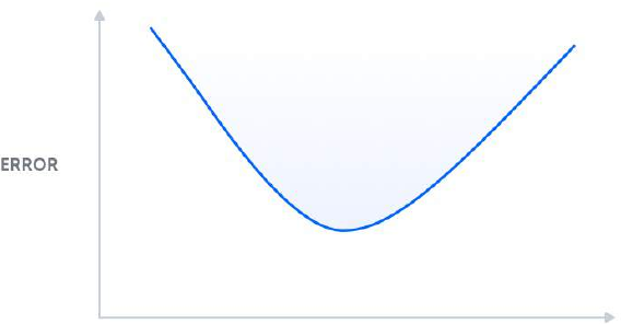
均方误差曲线

---

Step 4 — Building a Deep Q-learning Agent for Frozen Lake
In reinforcement learning, the neural network effectively predicts the
value of Q based on the state and action inputs, using a table to store
all the possible values, but this becomes unstable in complex games.
Deep
 reinforcement learning instead uses a neural network to
approximate the Q-function. For more details, see Understanding Deep
Q-Learning.
To get accustomed to Tensorflow, a deep learning library you installed
in Step 1, you will reimplement all of the logic used so far with
Tensorflow’s
 abstractions
 and
 you’ll
 use
 a
 neural network to
approximate your Q-function. However, your neural network will be
extremely simple: your output Q(s) is a matrix W multiplied by your
input s. This is known as a neural network with one fully-connected
layer:
Q(s) = Ws
To reiterate, the goal is to reimplement all of the logic from the bots
we’ve already built using Tensorflow’s abstractions. This will make your
operations
 more
 efficient,
 as
 Tensorflow
 can
 then
 perform all
computation on the GPU.
Begin by duplicating your Q-table script from Step 3:
cp bot_3_q_table.py bot_4_q_network.py
Then open the new file with nano or your preferred text editor:
nano bot_4_q_network.py
First, update the comment at the top of the file:
/AtariBot/bot_4_q_network.py
"""
Bot 4 -- Use Q-learning network to train bot
"""
. . .
Next, import the Tensorflow package by adding an import directive
right
 below import random.
 Additionally,
 add
tf.set_radon_seed(0) right below np.random.seed(0). This will
ensure that the results of this script will be repeatable across all sessions:
/AtariBot/bot_4_q_network.py
. . .
import random
import tensorflow as tf
random.seed(0)
np.random.seed(0)
tf.set_random_seed(0)
. . .
Redefine your hyperparameters at the top of the file to match the
following and add a function called exploration_probability,
which will return the probability of exploration at each step. Remember
that, in this context, “exploration” means taking a random action, as
opposed to taking the action recommended by the Q-value estimates:
/AtariBot/bot_4_q_network.py
. . .
num_episodes = 4000
discount_factor = 0.99
learning_rate = 0.15
report_interval = 500
exploration_probability = lambda episode: 50. / (episode + 10)
report = '100-ep Average: %.2f . Best 100-ep Average: %.2f . Average:
%.2f ' \
'(Episode %d)'
. . .
Next, you will add a one-hot encoding function. In short, one-hot
encoding is a process through which variables are converted into a form
that helps machine learning algorithms make better predictions. If you’d
like to learn more about one-hot encoding, you can check out Adversarial
Examples in Computer Vision: How to Build then Fool an Emotion-Based
Dog Filter.
Directly beneath report = ..., add a one_hot function:
/AtariBot/bot_4_q_network.py
. . .
report = '100-ep Average: %.2f . Best 100-ep Average: %.2f . Average:
%.2f ' \
'(Episode %d)'
def one_hot(i: int, n: int) -> np.array:
"""Implements one-hot encoding by selecting the ith standard basis
vector"""
return np.identity[i].reshape((1, -1))
def print_report(rewards: List, episode: int):
. . .
Next, you will rewrite your algorithm logic using Tensorflow’s
abstractions. Before doing that, though, you’ll need to first create
placeholders for your data.
In
 your main function, directly beneath rewards=[], insert the
following highlighted content. Here, you define placeholders for your
observation at time t (as obs_t_ph) and time t+1 (as obs_tp1_ph), as
well as placeholders for your action, reward, and Q target:
/AtariBot/bot_4_q_network.py
. . .
def main():
env = gym.make('FrozenLake-v0') # create the game
env.seed(0) # make results reproducible
rewards = []
# 1. Setup placeholders
n_obs, n_actions = env.observation_space.n, env.action_space.n
obs_t_ph = tf.placeholder(shape=[1, n_obs], dtype=tf.float32)
obs_tp1_ph = tf.placeholder(shape=[1, n_obs], dtype=tf.float32)
act_ph = tf.placeholder(tf.int32, shape=())
rew_ph = tf.placeholder(shape=(), dtype=tf.float32)
q_target_ph = tf.placeholder(shape=[1, n_actions], dtype=tf.float32)
Q = np.zeros((env.observation_space.n, env.action_space.n))
for episode in range(1, num_episodes + 1):
. . .
Directly beneath the line beginning with q_target_ph =, insert the
following highlighted lines. This code starts your computation by
computing Q(s, a) for all a to make q_current and Q(s’, a’) for all a’ to
make q_target:
/AtariBot/bot_4_q_network.py
. . .
rew_ph = tf.placeholder(shape=(), dtype=tf.float32)
q_target_ph = tf.placeholder(shape=[1, n_actions], dtype=tf.float32)
# 2. Setup computation graph
W = tf.Variable(tf.random_uniform([n_obs, n_actions], 0, 0.01))
q_current = tf.matmul(obs_t_ph, W)
q_target = tf.matmul(obs_tp1_ph, W)
Q = np.zeros((env.observation_space.n, env.action_space.n))
for episode in range(1, num_episodes + 1):
. . .
Again directly beneath the last line you added, insert the following
higlighted code. The first two lines are equivalent to the line added in
Step 3 that computes Qtarget,
 where Qtarget = reward +
discount_factor * np.max(Q[state2, :]). The next two lines
set up your loss, while the last line computes the action that maximizes
your Q-value:
/AtariBot/bot_4_q_network.py
. . .
q_current = tf.matmul(obs_t_ph, W)
q_target = tf.matmul(obs_tp1_ph, W)
q_target_max = tf.reduce_max(q_target_ph, axis=1)
q_target_sa = rew_ph + discount_factor * q_target_max
q_current_sa = q_current[0, act_ph]
error = tf.reduce_sum(tf.square(q_target_sa - q_current_sa))
pred_act_ph = tf.argmax(q_current, 1)
Q = np.zeros((env.observation_space.n, env.action_space.n))
for episode in range(1, num_episodes + 1):
. . .
After setting up your algorithm and the loss function, define your
optimizer:
/AtariBot/bot_4_q_network.py
. . .
error = tf.reduce_sum(tf.square(q_target_sa - q_current_sa))
pred_act_ph = tf.argmax(q_current, 1)
# 3. Setup optimization
trainer =
tf.train.GradientDescentOptimizer(learning_rate=learning_rate)
update_model = trainer.minimize(error)
Q = np.zeros((env.observation_space.n, env.action_space.n))
for episode in range(1, num_episodes + 1):
. . .
Next, set up the body of the game loop. To do this, pass data to the
Tensorflow placeholders and Tensorflow’s abstractions will handle the
computation on the GPU, returning the result of the algorithm.
Start by deleting the old Q-table and logic. Specifically, delete the lines
that define Q (right before the for loop), noise (in the while loop),
action, Qtarget, and Q[state, action]. Rename state to obs_t
and state2 to obs_tp1 to align with the Tensorflow placeholders you
set previously. When finished, your for loop will match the following:
/AtariBot/bot_4_q_network.py
. . .
# 3. Setup optimization
trainer =
tf.train.GradientDescentOptimizer(learning_rate=learning_rate)
update_model = trainer.minimize(error)
for episode in range(1, num_episodes + 1):
obs_t = env.reset()
episode_reward = 0
while True:
obs_tp1, reward, done, _ = env.step(action)
episode_reward += reward
obs_t = obs_tp1
if done:
...
Directly above the for loop, add the following two highlighted lines.
These lines initialize a Tensorflow session which in turn manages the
resources needed to run operations on the GPU. The second line
initializes all the variables in your computation graph; for example,
initializing weights to 0 before updating them. Additionally, you will
nest the for loop within the with statement, so indent the entire for
loop by four spaces:
/AtariBot/bot_4_q_network.py
. . .
trainer =
tf.train.GradientDescentOptimizer(learning_rate=learning_rate)
update_model = trainer.minimize(error)
with tf.Session() as session:
session.run(tf.global_variables_initializer())
for episode in range(1, num_episodes + 1):
obs_t = env.reset()
...
Before
 the
 line
 reading obs_tp1, reward, done, _ =
env.step(action), insert the following lines to compute the action.
This code evaluates the corresponding placeholder and replaces the
action with a random action with some probability:
/AtariBot/bot_4_q_network.py
. . .
while True:
# 4. Take step using best action or random action
obs_t_oh = one_hot(obs_t, n_obs)
action = session.run(pred_act_ph, feed_dict={obs_t_ph:
obs_t_oh})[0]
if np.random.rand(1) < exploration_probability(episode):
action = env.action_space.sample()
. . .
After the line containing env.step(action), insert the following to
train the neural network in estimating your Q-value function:
/AtariBot/bot_4_q_network.py
. . .
obs_tp1, reward, done, _ = env.step(action)
# 5. Train model
obs_tp1_oh = one_hot(obs_tp1, n_obs)
q_target_val = session.run(q_target, feed_dict={
obs_tp1_ph: obs_tp1_oh
})
session.run(update_model, feed_dict={
obs_t_ph: obs_t_oh,
rew_ph: reward,
q_target_ph: q_target_val,
act_ph: action
})
episode_reward += reward
. . .
Your final file will match this source code:
/AtariBot/bot_4_q_network.py
"""
Bot 4 -- Use Q-learning network to train bot
"""
from typing import List
import gym
import numpy as np
import random
import tensorflow as tf
random.seed(0)
np.random.seed(0)
tf.set_random_seed(0)
num_episodes = 4000
discount_factor = 0.99
learning_rate = 0.15
report_interval = 500
exploration_probability = lambda episode: 50. / (episode + 10)
report = '100-ep Average: %.2f . Best 100-ep Average: %.2f . Average:
%.2f ' \
'(Episode %d)'
def one_hot(i: int, n: int) -> np.array:
"""Implements one-hot encoding by selecting the ith standard basis
vector"""
return np.identity[i].reshape((1, -1))
def print_report(rewards: List, episode: int):
"""Print rewards report for current episode
- Average for last 100 episodes
- Best 100-episode average across all time
- Average for all episodes across time
"""
print(report % (
np.mean(rewards[-100:]),
max([np.mean(rewards[i:i+100]) for i in range(len(rewards) -
100)]),
np.mean(rewards),
episode))
def main():
env = gym.make('FrozenLake-v0')
 # create the game
env.seed(0)
 # make results reproducible
rewards = []
# 1. Setup placeholders
n_obs, n_actions = env.observation_space.n, env.action_space.n
obs_t_ph = tf.placeholder(shape=[1, n_obs], dtype=tf.float32)
obs_tp1_ph = tf.placeholder(shape=[1, n_obs], dtype=tf.float32)
act_ph = tf.placeholder(tf.int32, shape=())
rew_ph = tf.placeholder(shape=(), dtype=tf.float32)
q_target_ph = tf.placeholder(shape=[1, n_actions], dtype=tf.float32)
# 2. Setup computation graph
W = tf.Variable(tf.random_uniform([n_obs, n_actions], 0, 0.01))
q_current = tf.matmul(obs_t_ph, W)
q_target = tf.matmul(obs_tp1_ph, W)
q_target_max = tf.reduce_max(q_target_ph, axis=1)
q_target_sa = rew_ph + discount_factor * q_target_max
q_current_sa = q_current[0, act_ph]
error = tf.reduce_sum(tf.square(q_target_sa - q_current_sa))
pred_act_ph = tf.argmax(q_current, 1)
# 3. Setup optimization
trainer =
tf.train.GradientDescentOptimizer(learning_rate=learning_rate)
update_model = trainer.minimize(error)
with tf.Session() as session:
session.run(tf.global_variables_initializer())
for episode in range(1, num_episodes + 1):
obs_t = env.reset()
episode_reward = 0
while True:
obs_t_oh})[0]
# 4. Take step using best action or random action
obs_t_oh = one_hot(obs_t, n_obs)
action = session.run(pred_act_ph, feed_dict={obs_t_ph:
if np.random.rand(1) < exploration_probability(episode):
action = env.action_space.sample()
obs_tp1, reward, done, _ = env.step(action)
# 5. Train model
obs_tp1_oh = one_hot(obs_tp1, n_obs)
q_target_val = session.run(q_target, feed_dict={
obs_tp1_ph: obs_tp1_oh
})
session.run(update_model, feed_dict={
obs_t_ph: obs_t_oh,
rew_ph: reward,
q_target_ph: q_target_val,
act_ph: action
})
episode_reward += reward
obs_t = obs_tp1
ifdone:
rewards.append(episode_reward)
if episode % report_interval == 0:
print_report(rewards, episode)
break
print_report(rewards, -1)
if __name__ == '__main__':
main()
Save the file, exit your editor, and run the script:
python bot_4_q_network.py
Your output will end with the following, exactly:
Output
100-ep Average: 0.11 . Best 100-ep Average: 0.11 . Average: 0.05
(Episode 500)
100-ep Average: 0.41 . Best 100-ep Average: 0.54 . Average: 0.19
(Episode 1000)
100-ep Average: 0.56 . Best 100-ep Average: 0.73 . Average: 0.31
(Episode 1500)
100-ep Average: 0.57 . Best 100-ep Average: 0.73 . Average: 0.36
(Episode 2000)
100-ep Average: 0.65 . Best 100-ep Average: 0.73 . Average: 0.41
(Episode 2500)
100-ep Average: 0.65 . Best 100-ep Average: 0.73 . Average: 0.43
(Episode 3000)
100-ep Average: 0.69 . Best 100-ep Average: 0.73 . Average: 0.46
(Episode 3500)
100-ep Average: 0.77 . Best 100-ep Average: 0.79 . Average: 0.48
(Episode 4000)
100-ep Average: 0.77 . Best 100-ep Average: 0.79 . Average: 0.48
(Episode -1)
You’ve now trained your very first deep Q-learning agent. For a game
as simple as FrozenLake, your deep Q-learning agent required 4000
episodes to train. Imagine if the game were far more complex. How
many training samples would that require to train? As it turns out, the
agent could require millions of samples. The number of samples required
is referred to as sample complexity, a concept explored further in the next
section.
Understanding Bias-Variance Tradeoffs
Generally speaking, sample complexity is at odds with model complexity
in machine learning:
1. Model complexity: One wants a sufficiently complex model to solve
their problem. For example, a model as simple as a line is not
sufficiently complex to predict a car’s trajectory.
2. Sample complexity: One would like a model that does not require
many samples. This could be because they have a limited access to
labeled data, an insufficient amount of computing power, limited
memory, etc.
Say we have two models, one simple and one extremely complex. For
both models to attain the same performance, bias-variance tells us that
the extremely complex model will need exponentially more samples to
train. Case in point: your neural network-based Q-learning agent
required 4000 episodes to solve FrozenLake. Adding a second layer to the
neural network agent quadruples the number of necessary training
episodes. With increasingly complex neural networks, this divide only
grows. To maintain the same error rate, increasing model complexity
increases the sample complexity exponentially. Likewise, decreasing
sample complexity decreases model complexity. Thus, we cannot
maximize model complexity and minimize sample complexity to our
heart’s desire.
We can, however, leverage our knowledge of this tradeoff. For a visual
interpretation
 of
 the
 mathematics
 behind
 the bias-variance
decomposition, see Understanding the Bias-Variance Tradeoff. At a high
level, the bias-variance decomposition is a breakdown of “true error”
into two components: bias and variance. We refer to “true error” as mean
squared error (MSE), which is the expected difference between our
predicted labels and the true labels. The following is a plot showing the
change of “true error” as model complexity increases:
Mean Squared Error curve