Python 机器学习

分类简介

分类可以定义为从观察到的值或给定的数据点预测类别或类别的过程。分类输出可以采用“黑色”或“白色”、“垃圾邮件”或“非垃圾邮件”等形式。

从数学上讲，分类是将输入变量 (X) 映射到输出变量 (Y) 的近似映射函数 (f) 的任务。它基本上属于监督机器学习，其中除了输入数据集外，还提供了目标。

分类问题的一个例子是电子邮件中的垃圾邮件检测。输出只能有两个类别：“垃圾邮件”和“非垃圾邮件”；因此，这是一种二元分类。

要实现此分类，我们首先需要训练分类器。对于此示例，“垃圾邮件”和“非垃圾邮件”电子邮件将用作训练数据。成功训练分类器后，它可用于检测未知电子邮件。

分类中的学习器类型

关于分类问题，我们有两种类型的学习器：

惰性学习器 (Lazy Learners)

顾名思义，这类学习器在存储训练数据后等待测试数据出现。只有在获得测试数据后才进行分类。它们在训练上花费的时间较少，但在预测上花费的时间较多。惰性学习器的例子有 K-近邻和基于案例的推理。

急切学习器 (Eager Learners)

与惰性学习器相反，急切学习器在存储训练数据后无需等待测试数据出现即可构建分类模型。它们在训练上花费的时间较多，但在预测上花费的时间较少。急切学习器的例子有决策树、朴素贝叶斯和人工神经网络 (ANN)。

在 Python 中构建分类器

Scikit-learn 是一个用于机器学习的 Python 库，可用于在 Python 中构建分类器。在 Python 中构建分类器的步骤如下：

步骤 1：导入必要的 Python 包

为了使用 scikit-learn 构建分类器，我们需要导入它。我们可以使用以下脚本导入它：

import sklearn

步骤 2：导入数据集

导入必要的包后，我们需要一个数据集来构建分类预测模型。我们可以从 scikit-learn 数据集导入它，也可以根据我们的要求使用其他数据集。我们将使用 scikit-learn 的乳腺癌威斯康星诊断数据库。我们可以使用以下脚本导入它：

from sklearn.datasets import load_breast_cancer

以下脚本将加载数据集：

data = load_breast_cancer()

我们还需要组织数据，这可以通过以下脚本完成：

label_names = data['target_names']
labels = data['target']
feature_names = data['feature_names']
features = data['data']

以下命令将打印我们数据库中标签的名称，即“恶性”和“良性”。

print(label_names)

上述命令的输出是标签的名称：

['malignant' 'benign']

这些标签映射到二进制值 0 和 1。恶性肿瘤用 0 表示，良性肿瘤用 1 表示。

这些标签的特征名称和特征值可以通过以下命令查看：

print(feature_names[0])

上述命令的输出是标签 0（即恶性肿瘤）的特征名称：

mean radius

同样，标签的特征名称可以如下生成：

print(feature_names[1])

上述命令的输出是标签 1（即良性肿瘤）的特征名称：

mean texture

我们可以使用以下命令打印这些标签的特征：

print(features[0])

这将给出以下输出：

[1.799e+01 1.038e+01 1.228e+02 1.001e+03 1.184e-01 2.776e-01 3.001e-01
 1.471e-01 2.419e-01 7.871e-02 1.095e+00 9.053e-01 8.589e+00 1.534e+02
 6.399e-03 4.904e-02 5.373e-02 1.587e-02 3.003e-02 6.193e-03 2.538e+01
 1.733e+01 1.846e+02 2.019e+03 1.622e-01 6.656e-01 7.119e-01 2.654e-01
 4.601e-01 1.189e-01]

我们可以使用以下命令打印这些标签的特征：

print(features[1])

这将给出以下输出：

[2.057e+01 1.777e+01 1.329e+02 1.326e+03 8.474e-02 7.864e-02 8.690e-02
 7.017e-02 1.812e-01 5.667e-02 5.435e-01 7.339e-01 3.398e+00 7.408e+01
 5.225e-03 1.308e-02 1.860e-02 1.340e-02 1.389e-02 3.532e-03 2.499e+01
 2.341e+01 1.588e+02 1.956e+03 1.238e-01 1.866e-01 2.416e-01 1.860e-01
 2.750e-01 8.902e-02]

步骤 3：将数据组织成训练集和测试集

由于我们需要在未见过的数据上测试我们的模型，因此我们将数据集分为两部分：训练集和测试集。我们可以使用 scikit-learn Python 包的 train_test_split() 函数将数据拆分为集合。以下命令将导入该函数：

from sklearn.model_selection import train_test_split

现在，下一个命令将把数据拆分为训练数据和测试数据。在此示例中，我们使用 40% 的数据用于测试目的，60% 的数据用于训练目的：

train, test, train_labels, test_labels = train_test_split(features,labels,test_size = 0.40, random_state = 42)

步骤 4：模型评估

将数据分成训练集和测试集后，我们需要构建模型。我们将为此目的使用朴素贝叶斯算法。以下命令将导入 GaussianNB 模块：

from sklearn.naive_bayes import GaussianNB

现在，如下初始化模型：

gnb = GaussianNB()

接下来，借助以下命令，我们可以训练模型：

model = gnb.fit(train, train_labels)

现在，为了评估目的，我们需要进行预测。这可以通过使用 predict() 函数来完成，如下所示：

preds = gnb.predict(test)
print(preds)

这将给出以下输出：

[1 0 0 1 1 0 0 0 1 1 1 0 1 0 1 0 1 1 1 0 1 1 0 1 1 1 1 1 1 0 1 1 1 1 1 1 0
 1 0 1 1 0 1 1 1 1 1 1 1 1 0 0 1 1 1 1 1 0 0 1 1 0 0 1 1 1 0 0 1 1 0 0 1 0
 1 1 1 1 1 1 0 1 1 0 0 0 0 0 1 1 1 1 1 1 1 1 0 0 1 0 0 1 0 0 1 1 1 0 1 1 0
 1 1 0 0 0 1 1 1 0 0 1 1 0 1 0 0 1 1 0 0 0 1 1 1 0 1 1 0 0 1 0 1 1 0 1 0 0
 1 1 1 1 1 1 1 0 0 1 1 1 1 1 1 1 1 1 1 1 1 0 1 1 1 0 1 1 0 1 1 1 1 1 1 0 0
 0 1 1 0 1 0 1 1 1 1 0 1 1 0 1 1 1 0 1 0 0 1 1 1 1 1 1 1 1 0 1 1 1 1 1 0 1
 0 0 1 1 0 1]

输出中上面的一系列 0 和 1 是恶性肿瘤和良性肿瘤类别的预测值。

步骤 5：查找准确性

我们可以通过比较 test_labels 和 preds 两个数组来找到上一步构建的模型的准确性。我们将使用 accuracy_score() 函数来确定准确性。

from sklearn.metrics import accuracy_score
print(accuracy_score(test_labels,preds))

0.951754385965

上述输出表明朴素贝叶斯分类器的准确率为 95.17%。

分类评估指标

即使您已经完成了机器学习应用程序或模型的实现，工作也没有完成。我们必须找出我们的模型有多有效？可能有不同的评估指标，但我们必须仔细选择它们，因为指标的选择会影响机器学习算法的性能如何衡量和比较。

以下是一些重要的分类评估指标，您可以根据数据集和问题类型进行选择：

混淆矩阵 (Confusion Matrix)

这是衡量分类问题性能的最简单方法，其中输出可以是两种或更多种类型。混淆矩阵只是一张具有两个维度（即“实际”和“预测”）的表格，此外，这两个维度都有“真阳性 (TP)”、“真阴性 (TN)”、“假阳性 (FP)”、“假阴性 (FN)”，如下所示：

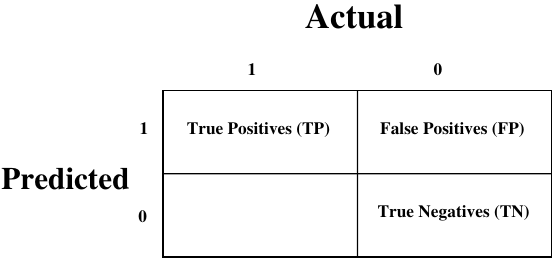
与混淆矩阵相关的术语解释如下：

• 真阳性 (TP)： 指数据点的实际类别和预测类别均为 1 的情况。
• 真阴性 (TN)： 指数据点的实际类别和预测类别均为 0 的情况。
• 假阳性 (FP)： 指数据点的实际类别为 0 但预测类别为 1 的情况。
• 假阴性 (FN)： 指数据点的实际类别为 1 但预测类别为 0 的情况。

我们可以借助 sklearn 的 confusion_matrix() 函数找到混淆矩阵。借助以下脚本，我们可以找到上面构建的二元分类器的混淆矩阵：

from sklearn.metrics import confusion_matrix
print(confusion_matrix(test_labels,preds)) # 完整的代码会在此处显示，但原文本省略了它

输出

[[ 73   7]
 [  4 144]]

准确率 (Accuracy)

它可以定义为我们的机器学习模型做出的正确预测的数量。我们可以借助以下公式通过混淆矩阵轻松计算它：

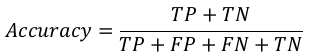
对于上面构建的二元分类器，TP + TN = 73 + 144 = 217，TP + FP + FN + TN = 73 + 7 + 4 + 144 = 228。

因此，准确率 = 217 / 228 = 0.951754385965，这与我们创建二元分类器后计算的结果相同。

精确率 (Precision)

精确率，用于文档检索，可以定义为我们的机器学习模型返回的正确文档的数量。我们可以借助以下公式通过混淆矩阵轻松计算它：

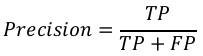
对于上面构建的二元分类器，TP = 73，TP + FP = 73 + 7 = 80。

因此，精确率 = 73 / 80 = 0.915。

召回率或灵敏度 (Recall or Sensitivity)

召回率可以定义为我们的机器学习模型返回的阳性数量。我们可以借助以下公式通过混淆矩阵轻松计算它：

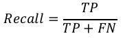
对于上面构建的二元分类器，TP = 73，TP + FN = 73 + 4 = 77。

因此，召回率 = 73 / 77 = 0.94805。

特异度 (Specificity)

特异度与召回率相反，可以定义为我们的机器学习模型返回的阴性数量。我们可以借助以下公式通过混淆矩阵轻松计算它：

对于上面构建的二元分类器，TN = 144，TN + FP = 144 + 7 = 151。

因此，特异度 = 144 / 151 = 0.95364。

各种机器学习分类算法

以下是一些重要的机器学习分类算法：

• 逻辑回归 (Logistic Regression)
• 支持向量机 (Support Vector Machine, SVM)
• 决策树 (Decision Tree)
• 朴素贝叶斯 (Naïve Bayes)
• 随机森林 (Random Forest)

我们将在后续章节中详细讨论所有这些分类算法。

应用

分类算法的一些最重要的应用如下：

• 语音识别 (Speech Recognition)
• 手写识别 (Handwriting Recognition)
• 生物识别 (Biometric Identification)
• 文档分类 (Document Classification)

9. Classification – Introduction
 Machine Learning with Python
Introduction to Classification
Classification may be defined as the process of predicting class or category from observed
values or given data points. The categorized output can have the form such as “Black” or
“White” or “spam” or “no spam”.
Mathematically, classification is the task of approximating a mapping function (f) from
input variables (X) to output variables (Y). It is basically belongs to the supervised machine
learning in which targets are also provided along with the input data set.
An example of classification problem can be the spam detection in emails. There can be
only two categories of output, “spam” and “no spam”; hence this is a binary type
classification.
To implement this classification, we first need to train the classifier. For this example,
“spam” and “no spam” emails would be used as the training data. After successfully train
the classifier, it can be used to detect an unknown email.
Types of Learners in Classification
We have two types of learners in respective to classification problems:
Lazy Learners
As the name suggests, such kind of learners waits for the testing data to be appeared after
storing the training data. Classification is done only after getting the testing data. They
spend less time on training but more time on predicting. Examples of lazy learners are K-
nearest neighbor and case-based reasoning.
Eager Learners
As opposite to lazy learners, eager learners construct classification model without waiting
for the testing data to be appeared after storing the training data. They spend more time
on training but less time on predicting. Examples of eager learners are Decision Trees,
Naïve Bayes and Artificial Neural Networks (ANN).
Building a Classifier in Python
Scikit-learn, a Python library for machine learning can be used to build a classifier in
Python. The steps for building a classifier in Python are as follows:
Step1: Importing necessary python package
For building a classifier using scikit-learn, we need to import it. We can import it by using
following script:
57
import sklearn
Machine Learning with Python
Step2: Importing dataset
After importing necessary package, we need a dataset to build classification prediction
model. We can import it from sklearn dataset or can use other one as per our requirement.
We are going to use sklearn’s Breast Cancer Wisconsin Diagnostic Database. We can
import it with the help of following script:
from sklearn.datasets import load_breast_cancer
The following script will load the dataset;
data = load_breast_cancer()
We also need to organize the data and it can be done with the help of following scripts:
label_names = data['target_names']
labels = data['target']
feature_names = data['feature_names']
features = data['data']
The following command will print the name of the labels, ‘malignant’ and ‘benign’ in
case of our database.
print(label_names)
The output of the above command is the names of the labels:
['malignant' 'benign']
These labels are mapped to binary values 0 and 1. Malignant cancer is represented by 0
and Benign cancer is represented by 1.
The feature names and feature values of these labels can be seen with the help of following
commands:
print(feature_names[0])
The output of the above command is the names of the features for label 0 i.e. Malignant
cancer:
mean radius
Similarly, names of the features for label can be produced as follows:
print(feature_names[1])
58
Machine Learning with Python
The output of the above command is the names of the features for label 1 i.e. Benign
cancer:
mean texture
We can print the features for these labels with the help of following command:
print(features[0])
This will give the following output:
[1.799e+01 1.038e+01 1.228e+02 1.001e+03 1.184e-01 2.776e-01 3.001e-01
1.471e-01 2.419e-01 7.871e-02 1.095e+00 9.053e-01 8.589e+00 1.534e+02
6.399e-03 4.904e-02 5.373e-02 1.587e-02 3.003e-02 6.193e-03 2.538e+01
1.733e+01 1.846e+02 2.019e+03 1.622e-01 6.656e-01 7.119e-01 2.654e-01
4.601e-01 1.189e-01]
We can print the features for these labels with the help of following command:
print(features[1])
This will give the following output:
[2.057e+01 1.777e+01 1.329e+02 1.326e+03 8.474e-02 7.864e-02 8.690e-02
7.017e-02 1.812e-01 5.667e-02 5.435e-01 7.339e-01 3.398e+00 7.408e+01
5.225e-03 1.308e-02 1.860e-02 1.340e-02 1.389e-02 3.532e-03 2.499e+01
2.341e+01 1.588e+02 1.956e+03 1.238e-01 1.866e-01 2.416e-01 1.860e-01
2.750e-01 8.902e-02]
Step3: Organizing data into training & testing sets
As we need to test our model on unseen data, we will divide our dataset into two parts: a
training set and a test set. We can use train_test_split() function of sklearn python
package to split the data into sets. The following command will import the function:
from sklearn.model_selection import train_test_split
Now, next command will split the data into training & testing data. In this example, we
are using taking 40 percent of the data for testing purpose and 60 percent of the data for
training purpose:
train, test, train_labels, test_labels =
train_test_split(features,labels,test_size = 0.40, random_state = 42)
59
Machine Learning with Python
Step4- Model evaluation
After dividing the data into training and testing we need to build the model. We will be
using Naïve Bayes algorithm for this purpose. The following commands will import the
GaussianNB module:
from sklearn.naive_bayes import GaussianNB
Now, initialize the model as follows:
gnb = GaussianNB()
Next, with the help of following command we can train the model:
model = gnb.fit(train, train_labels)
Now, for evaluation purpose we need to make predictions. It can be done by using
predict() function as follows:
preds = gnb.predict(test)
print(preds)
This will give the following output:
[1 0 0 1 1 0 0 0 1 1 1 0 1 0 1 0 1 1 1 0 1 1 0 1 1 1 1 1 1 0 1 1 1 1 1 1 0
1 0 1 1 0 1 1 1 1 1 1 1 1 0 0 1 1 1 1 1 0 0 1 1 0 0 1 1 1 0 0 1 1 0 0 1 0
1 1 1 1 1 1 0 1 1 0 0 0 0 0 1 1 1 1 1 1 1 1 0 0 1 0 0 1 0 0 1 1 1 0 1 1 0
1 1 0 0 0 1 1 1 0 0 1 1 0 1 0 0 1 1 0 0 0 1 1 1 0 1 1 0 0 1 0 1 1 0 1 0 0
1 1 1 1 1 1 1 0 0 1 1 1 1 1 1 1 1 1 1 1 1 0 1 1 1 0 1 1 0 1 1 1 1 1 1 0 0
0 1 1 0 1 0 1 1 1 1 0 1 1 0 1 1 1 0 1 0 0 1 1 1 1 1 1 1 1 0 1 1 1 1 1 0 1
0 0 1 1 0 1]
The above series of 0s and 1s in output are the predicted values for the Malignant and
Benign tumor classes.
Step5- Finding accuracy
We can find the accuracy of the model build in previous step by comparing the two arrays
namely test_labels and preds. We will be using the accuracy_score() function to
determine the accuracy.
from sklearn.metrics import accuracy_score
print(accuracy_score(test_labels,preds))
0.951754385965
The above output shows that NaïveBayes classifier is 95.17% accurate.
60
Machine Learning with Python
Classification Evaluation Metrics
The job is not done even if you have finished implementation of your Machine Learning
application or model. We must have to find out how effective our model is? There can be
different evaluation metrics, but we must choose it carefully because the choice of metrics
influences how the performance of a machine learning algorithm is measured and
compared.
The following are some of the important classification evaluation metrics among which you
can choose based upon your dataset and kind of problem:
Confusion Matrix
It is the easiest way to measure the performance of a classification problem where the
output can be of two or more type of classes. A confusion matrix is nothing but a table
with two dimensions viz. “Actual” and “Predicted” and furthermore, both the dimensions
have “True Positives (TP)”, “True Negatives (TN)”, “False Positives (FP)”, “False Negatives
(FN)” as shown below:
Predicted
1
0
Actual
1
 0
True Positives (TP)
 False Positives (FP)
False Negatives (FN)
 True Negatives (TN)
The explanation of the terms associated with confusion matrix are as follows:

 True Positives (TP): It is the case when both actual class & predicted class of
data point is 1.

True Negatives (TN): It is the case when both actual class & predicted class of
data point is 0.

False Positives (FP): It is the case when actual class of data point is 0 & predicted
class of data point is 1.

False Negatives (FN): It is the case when actual class of data point is 1 &
predicted class of data point is 0.
We can find the confusion matrix with the help of confusion_matrix() function of
sklearn. With the help of the following script, we can find the confusion matrix of above
built binary classifier:
61
Machine Learning with Python
from sklearn.metrics import confusion_matrix
Output
[[ 73
 7]
[
 4 144]]
Accuracy
It may be defined as the number of correct predictions made by our ML model. We can
easily calculate it by confusion matrix with the help of following formula:
TP + TN
Accuracy =
TP + FP + FN + TN
For above built binary classifier, TP + TN = 73+144 = 217 and TP+FP+FN+TN =
73+7+4+144=228.
Hence, Accuracy = 217/228 = 0.951754385965 which is same as we have calculated after
creating our binary classifier.
Precision
Precision, used in document retrievals, may be defined as the number of correct
documents returned by our ML model. We can easily calculate it by confusion matrix with
the help of following formula:
TP
Precision =
TP + FP
For the above built binary classifier, TP = 73 and TP+FP = 73+7 = 80.
Hence, Precision = 73/80 = 0.915
Recall or Sensitivity
Recall may be defined as the number of positives returned by our ML model. We can easily
calculate it by confusion matrix with the help of following formula:
TP
Recall =
TP + FN
62
Machine Learning with Python
For above built binary classifier, TP = 73 and TP+FN = 73+4 = 77.
Hence, Precision = 73/77 = 0.94805
Specificity
Specificity, in contrast to recall, may be defined as the number of negatives returned by
our ML model. We can easily calculate it by confusion matrix with the help of following
formula:
TN
Specificity =
TN + FP
For the above built binary classifier, TN = 144 and TN+FP = 144+7 = 151.
Hence, Precision = 144/151 = 0.95364
Various ML Classification Algorithms
The followings are some important ML classification algorithms:

 Logistic Regression

 Support Vector Machine (SVM)

 Decision Tree

 Naïve Bayes

 Random Forest
We will be discussing all these classification algorithms in detail in further chapters.
Applications
Some of the most important applications of classification algorithms are as follows:

 Speech Recognition

 Handwriting Recognition

 Biometric Identification

 Document Classification