Python 机器学习
逻辑回归简介
逻辑回归是一种监督学习分类算法,用于预测目标变量的概率。目标变量或因变量的性质是二分法的,这意味着只有两个可能的类别。
简单来说,因变量本质上是二元的,数据编码为 1(表示成功/是)或 0(表示失败/否)。
从数学上讲,逻辑回归模型将 P(Y=1) 预测为 X 的函数。它是最简单的机器学习算法之一,可用于各种分类问题,例如垃圾邮件检测、糖尿病预测、癌症检测等。
逻辑回归的类型
通常,逻辑回归指的是具有二元目标变量的二元逻辑回归,但它还可以预测另外两种类别的目标变量。根据类别的数量,逻辑回归可以分为以下类型:
二元或二项式 (Binary or Binomial)
在这种分类中,因变量只有两种可能的类型,即 1 和 0。例如,这些变量可以表示成功或失败、是或否、赢或输等。
多项式 (Multinomial)
在这种分类中,因变量可以有 3 种或更多种可能的无序类型,即没有定量意义的类型。例如,这些变量可以表示“A 型”或“B 型”或“C 型”。
有序 (Ordinal)
在这种分类中,因变量可以有 3 种或更多种可能的有序类型,即具有定量意义的类型。例如,这些变量可以表示“差”、“好”、“非常好”、“优秀”,并且每个类别可以有 0、1、2、3 等分数。
逻辑回归假设
在深入了解逻辑回归的实现之前,我们必须了解以下有关它的假设:
- 对于二元逻辑回归,目标变量必须始终是二元的,并且期望的结果由因子水平 1 表示。
- 模型中不应存在任何多重共线性,这意味着自变量必须相互独立。
- 我们必须在模型中包含有意义的变量。
- 对于逻辑回归,我们应该选择大的样本量。
二元逻辑回归模型
逻辑回归最简单的形式是二元或二项式逻辑回归,其中目标变量或因变量只有 2 种可能的类型,即 1 或 0。它允许我们对多个预测变量和二元/二项式目标变量之间的关系进行建模。在逻辑回归的情况下,线性函数基本上用作另一个函数的输入,例如以下关系中的 g:
![]() hθ(x)=g(θTx)其中 0≤hθ≤1这里,g 是逻辑或 Sigmoid 函数,
hθ(x)=g(θTx)其中 0≤hθ≤1这里,g 是逻辑或 Sigmoid 函数,
可以表示为: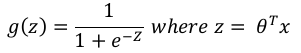 g(z)=1+e−Z1其中 z=θTx
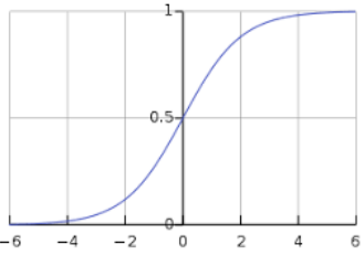
Sigmoid 曲线可以通过以下图表表示。我们可以看到 y 轴的值介于 0 和 1 之间,并在 0.5 处穿过轴。
这些类别可以分为正类或负类。如果输出介于 0 和 1 之间,则它属于正类的概率。对于我们的实现,如果假设函数的输出 ge0.5,我们将其解释为正,否则为负。
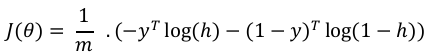
我们还需要定义一个损失函数来衡量算法在使用函数上的权重(由 theta 表示)的性能,如下所示:
h=g(Xθ)
现在,在定义了损失函数之后,我们的首要目标是最小化损失函数。这可以通过拟合权重来完成,这意味着通过增加或减少权重。借助损失函数对每个权重的导数,我们将能够知道哪些参数应该具有高权重,哪些应该具有较小的权重。
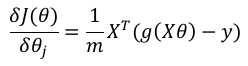
以下梯度下降方程告诉我们如果修改参数,损失将如何变化:
在 Python 中实现
现在我们将在 Python 中实现上述二项式逻辑回归的概念。为此,我们使用一个多变量花卉数据集,名为“iris”,它有 3 个类别,每个类别 50 个实例,但我们将使用前两个特征列。每个类别代表一种鸢尾花。
首先,我们需要导入必要的库,如下所示:
import numpy as np
import matplotlib.pyplot as plt
import seaborn as sns # 这个库虽然导入了,但在后续代码中没有直接使用

from sklearn import datasets
接下来,加载鸢尾花数据集,如下所示:
iris = datasets.load_iris()
X = iris.data[:, :2] # 只取前两个特征
y = (iris.target != 0) * 1 # 将目标变量转换为二元,0类为0,其他类为1
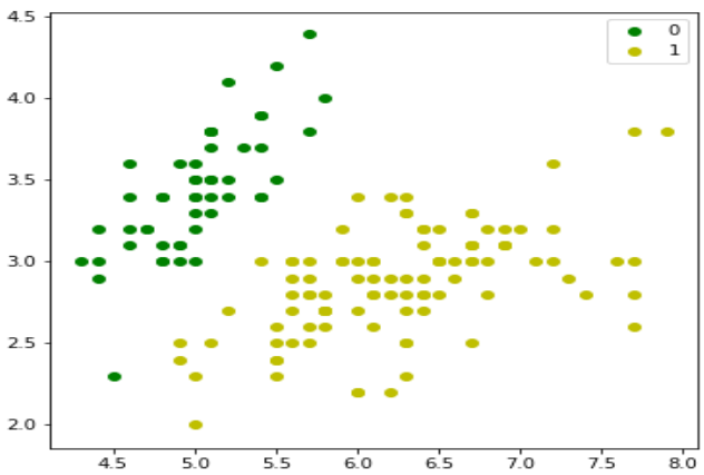
我们可以绘制我们的训练数据,如下所示:
plt.figure(figsize=(6, 6))
plt.scatter(X[y == 0][:, 0], X[y == 0][:, 1], color='g', label='0')
plt.scatter(X[y == 1][:, 0], X[y == 1][:, 1], color='y', label='1')
plt.legend()
plt.show() # 添加这一行以显示图形
接下来,我们将定义 Sigmoid 函数、损失函数和梯度下降,如下所示:
class LogisticRegression:
    def __init__(self, lr=0.01, num_iter=100000, fit_intercept=True, verbose=False):
        self.lr = lr
        self.num_iter = num_iter
        self.fit_intercept = fit_intercept
        self.verbose = verbose

    def __add_intercept(self, X):
        intercept = np.ones((X.shape[0], 1))
        return np.concatenate((intercept, X), axis=1)

    def __sigmoid(self, z):
        return 1 / (1 + np.exp(-z))

    def __loss(self, h, y):
        # 使用np.mean来计算平均损失,并处理log(0)的情况
        return -np.mean(y * np.log(h + 1e-10) + (1 - y) * np.log(1 - h + 1e-10))

    def fit(self, X, y):
        if self.fit_intercept:
            X = self.__add_intercept(X)

        # 现在,初始化权重,如下所示:
        self.theta = np.zeros(X.shape[1])

        for i in range(self.num_iter):
            z = np.dot(X, self.theta)
            h = self.__sigmoid(z)
            gradient = np.dot(X.T, (h - y)) / y.size
            self.theta -= self.lr * gradient

            if(self.verbose == True and i % 10000 == 0):
                loss = self.__loss(h, y) # 在 verbose 模式下计算损失
                print(f'loss: {loss} \t')

    # 借助以下脚本,我们可以预测输出概率:
    def predict_prob(self, X):
        if self.fit_intercept:
            X = self.__add_intercept(X)
        return self.__sigmoid(np.dot(X, self.theta))

    def predict(self, X):
        return self.predict_prob(X).round()
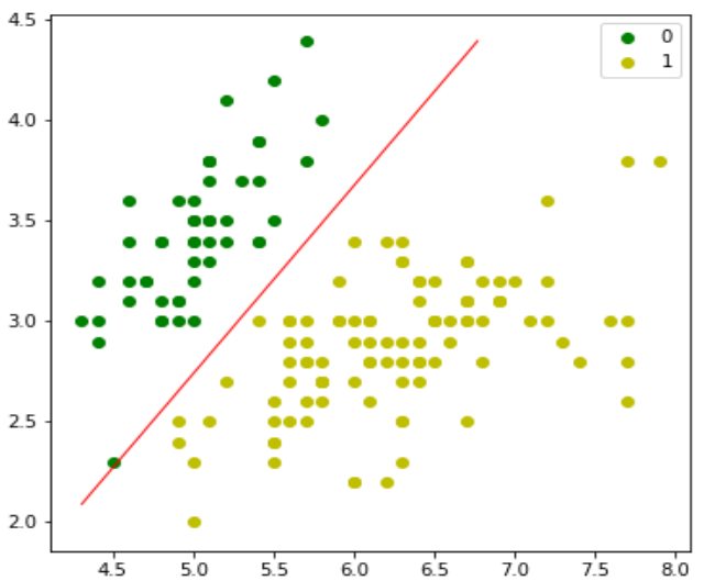
接下来,我们可以评估模型并绘制它,如下所示:
model = LogisticRegression(lr=0.1, num_iter=300000)
model.fit(X, y) # 调用fit方法进行训练
preds = model.predict(X)
print(f"Accuracy: {(preds == y).mean()}")

plt.figure(figsize=(10, 6))
plt.scatter(X[y == 0][:, 0], X[y == 0][:, 1], color='g', label='0')
plt.scatter(X[y == 1][:, 0], X[y == 1][:, 1], color='y', label='1')
plt.legend()

x1_min, x1_max = X[:,0].min() - 1, X[:,0].max() + 1 # 增加一些边界
x2_min, x2_max = X[:,1].min() - 1, X[:,1].max() + 1 # 增加一些边界
xx1, xx2 = np.meshgrid(np.linspace(x1_min, x1_max, 100), np.linspace(x2_min, x2_max, 100)) # 增加网格点密度
grid = np.c_[xx1.ravel(), xx2.ravel()]
probs = model.predict_prob(grid).reshape(xx1.shape)

plt.contour(xx1, xx2, probs, [0.5], linewidths=1, colors='red')
plt.show() # 添加这一行以显示图形
多项式逻辑回归模型 (Multinomial Logistic Regression Model)
逻辑回归的另一种有用形式是多项式逻辑回归,其中目标变量或因变量可以有 3 种或更多种可能的无序类型,即没有定量意义的类型。
在 Python 中实现
现在我们将在 Python 中实现上述多项式逻辑回归的概念。为此,我们使用来自 sklearn 的名为 digit 的数据集。
首先,我们需要导入必要的库,如下所示:
from sklearn import datasets
from sklearn import linear_model
from sklearn import metrics
from sklearn.model_selection import train_test_split
接下来,我们需要加载 digit 数据集:
digits = datasets.load_digits()
现在,如下定义特征矩阵(X)和响应向量:
X = digits.data
y = digits.target
借助下一行代码,我们可以将 X 和 y 拆分为训练集和测试集:
X_train, X_test, y_train, y_test = train_test_split(X, y,
                                                    test_size=0.4,
                                                    random_state=1)
现在,如下创建一个逻辑回归对象:
digreg = linear_model.LogisticRegression(max_iter=10000, solver='liblinear') # 增加 max_iter 并指定 solver 以避免收敛警告
现在,我们需要使用训练集来训练模型,如下所示:
digreg.fit(X_train, y_train)
接下来,对测试集进行预测,如下所示:
y_pred = digreg.predict(X_test)
接下来打印模型的准确率,如下所示:
print("Accuracy of Logistic Regression model is:",
      metrics.accuracy_score(y_test, y_pred)*100)
输出
Accuracy of Logistic Regression model is: 95.6884561891516
从上面的输出中我们可以看到,我们模型的准确率约为 96%。
10. Classification Algorithms – Logistic
Machine Learning Regression
with Python
Introduction to Logistic Regression
Logistic regression is a supervised learning classification algorithm used to predict the
probability of a target variable. The nature of target or dependent variable is dichotomous,
which means there would be only two possible classes.
In simple words, the dependent variable is binary in nature having data coded as either 1
(stands for success/yes) or 0 (stands for failure/no).
Mathematically, a logistic regression model predicts P(Y=1) as a function of X. It is one of
the simplest ML algorithms that can be used for various classification problems such as
spam detection, Diabetes prediction, cancer detection etc.
Types of Logistic Regression
Generally, logistic regression means binary logistic regression having binary target
variables, but there can be two more categories of target variables that can be predicted
by it. Based on those number of categories, Logistic regression can be divided into
following types:
Binary or Binomial
In such a kind of classification, a dependent variable will have only two possible types
either 1 and 0. For example, these variables may represent success or failure, yes or no,
win or loss etc.
Multinomial
In such a kind of classification, dependent variable can have 3 or more possible unordered
types or the types having no quantitative significance. For example, these variables may
represent “Type A” or “Type B” or “Type C”.
Ordinal
In such a kind of classification, dependent variable can have 3 or more possible ordered
types or the types having a quantitative significance. For example, these variables may
represent “poor” or “good”, “very good”, “Excellent” and each category can have the scores
like 0,1,2,3.
Logistic Regression Assumptions
Before diving into the implementation of logistic regression, we must be aware of the
following assumptions about the same:
64
Machine Learning with Python
In case of binary logistic regression, the target variables must be binary always
and the desired outcome is represented by the factor level 1.
There should not be any multi-collinearity in the model, which means
the
independent variables must be independent of each other.
We must include meaningful variables in our model.
We should choose a large sample size for logistic regression.
Binary Logistic Regression model
The simplest form of logistic regression is binary or binomial logistic regression in which
the target or dependent variable can have only 2 possible types either 1 or 0. It allows us
to model a relationship between multiple predictor variables and a binary/binomial target
variable. In case of logistic regression, the linear function is basically used as an input to
another function such as g in the following relation:
hθ (x) = g(θT x)where 0 ≤ hθ ≤ 1
Here, g is the logistic or sigmoid function which can be given as follows:
1
g(z) =
where z = θ T x
1 + e−Z
To sigmoid curve can be represented with the help of following graph. We can see the
values of y-axis lie between 0 and 1 and crosses the axis at 0.5.
The classes can be divided into positive or negative. The output comes under the
probability of positive class if it lies between 0 and 1. For our implementation, we are
interpreting the output of hypothesis function as positive if it is ≥ 0.5, otherwise negative.
We also need to define a loss function to measure how well the algorithm performs using
the weights on functions, represented by theta as follows:
h = g(Xθ)
J(θ) =
1
m
. (−yT log − (1 − y)T log(1 − h))
65
Machine Learning with Python
Now, after defining the loss function our prime goal is to minimize the loss function. It can
be done with the help of fitting the weights which means by increasing or decreasing the
weights. With the help of derivatives of the loss function w.r.t each weight, we would be
able to know what parameters should have high weight and what should have smaller
weight.
The following gradient descent equation tells us how loss would change if we modified the
parameters:
δJ(θ) 1= X T
(g(Xθ) − y)
δθ j
m
Implementation in Python
Now we will implement the above concept of binomial logistic regression in Python. For
this purpose, we are using a multivariate flower dataset named ‘iris’ which have 3 classes
of 50 instances each, but we will be using the first two feature columns. Every class
represents a type of iris flower.
First, we need to import the necessary libraries as follows:
import numpy as np
import matplotlib.pyplot as plt
import seaborn as sns
from sklearn import datasets
Next, load the iris dataset as follows:
iris = datasets.load_iris()
X = iris.data[:, :2]
y = (iris.target != 0) * 1
We can plot our training data s follows:
plt.figure(figsize=(6, 6))
plt.scatter(X[y == 0][:, 0], X[y == 0][:, 1], color='g', label='0')
plt.scatter(X[y == 1][:, 0], X[y == 1][:, 1], color='y', label='1')
plt.legend();
66
Machine Learning with Python
Next, we will define sigmoid function, loss function and gradient descend as follows:
class LogisticRegression:
def __init__(self, lr=0.01, num_iter=100000, fit_intercept=True,
verbose=False):
self.lr = lr
self.num_iter = num_iter
self.fit_intercept = fit_intercept
self.verbose = verbose
def __add_intercept(self, X):
intercept = np.ones((X.shape[0], 1))
return np.concatenate((intercept, X), axis=1)
def __sigmoid(self, z):
return 1 / (1 + np.exp(-z))
def __loss(self, h, y):
return (-y * np.log - (1 - y) * np.log(1 - h)).mean()
def fit(self, X, y):
if self.fit_intercept:
X = self.__add_intercept(X)
67
Machine Learning with Python
Now, initialize the weights as follows:
self.theta = np.zeros(X.shape[1])
for i in range(self.num_iter):
z = np.dot(X, self.theta)
h = self.__sigmoid(z)
gradient = np.dot(X.T, (h - y)) / y.size
self.theta -= self.lr * gradient
z = np.dot(X, self.theta)
h = self.__sigmoid(z)
loss = self.__loss(h, y)
if(self.verbose ==True and i % 10000 == 0):
print(f'loss: {loss} \t')
With the help of the following script, we can predict the output probabilities:
def predict_prob(self, X):
if self.fit_intercept:
X = self.__add_intercept(X)
return self.__sigmoid(np.dot(X, self.theta))
def predict(self, X):
return self.predict_prob(X).round()
Next, we can evaluate the model and plot it as follows:
model = LogisticRegression(lr=0.1, num_iter=300000)
preds = model.predict(X)
(preds == y).mean()
plt.figure(figsize=(10, 6))
plt.scatter(X[y == 0][:, 0], X[y == 0][:, 1], color='g', label='0')
plt.scatter(X[y == 1][:, 0], X[y == 1][:, 1], color='y', label='1')
plt.legend()
x1_min, x1_max = X[:,0].min(), X[:,0].max(),
x2_min, x2_max = X[:,1].min(), X[:,1].max(),
68
Machine Learning with Python
xx1, xx2 = np.meshgrid(np.linspace(x1_min, x1_max), np.linspace(x2_min,
x2_max))
grid = np.c_[xx1.ravel(), xx2.ravel()]
probs = model.predict_prob(grid).reshape(xx1.shape)
plt.contour(xx1, xx2, probs, [0.5], linewidths=1, colors='red');
Multinomial Logistic Regression Model
Another useful form of logistic regression is multinomial logistic regression in which the
target or dependent variable can have 3 or more possible unordered types i.e. the types
having no quantitative significance.
Implementation in Python
Now we will implement the above concept of multinomial logistic regression in Python.
For this purpose, we are using a dataset from sklearn named digit.
First, we need to import the necessary libraries as follows:
Import sklearn
from sklearn import datasets
from sklearn import linear_model
from sklearn import metrics
69
Machine Learning with Python
from sklearn.model_selection import train_test_split
Next, we need to load digit dataset:
digits = datasets.load_digits()
Now, define the feature matrix(X) and response vectoras follows:
X = digits.data
y = digits.target
With the help of next line of code, we can split X and y into training and testing sets:
X_train, X_test, y_train, y_test = train_test_split(X, y,
test_size=0.4,
random_state=
1)
Now create an object of logistic regression as follows:
digreg = linear_model.LogisticRegression()
Now, we need to train the model by using the training sets as follows:
digreg.fit(X_train, y_train)
Next, make the predictions on testing set as follows:
y_pred = digreg.predict(X_test)
Next print the accuracy of the model as follows:
print("Accuracy of Logistic Regression model is:",
metrics.accuracy_score(y_test, y_pred)*100)
Output
Accuracy of Logistic Regression model is: 95.6884561891516
From the above output we can see the accuracy of our model is around 96 percent.