Python 机器学习
SVM 简介
支持向量机 (SVM) 是强大而灵活的监督机器学习算法,用于分类和回归。但通常,它们用于分类问题。SVM 最初于 1960 年代提出,但后来在 1990 年代得到完善。与其他机器学习算法相比,SVM 具有独特的实现方式。最近,由于它们处理多个连续和分类变量的能力,它们变得非常流行。
SVM 的工作原理
SVM 模型本质上是多维空间中超平面中不同类别的表示。SVM 将以迭代方式生成超平面,以便最小化误差。SVM 的目标是将数据集划分为类别,以找到最大间隔超平面 (MMH)。
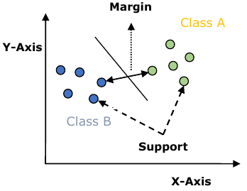
支持向量 (Support Vectors)
X 轴
Y 轴
类别 A
类别 B
间隔 (Margin)
以下是 SVM 中的重要概念:
- 支持向量 (Support Vectors):最接近超平面的数据点称为支持向量。分离线将借助这些数据点定义。
- 超平面 (Hyperplane):正如我们在上图中看到的,它是一个决策平面或空间,用于分隔具有不同类别的一组对象。
- 间隔 (Margin):它可以定义为不同类别最近数据点上的两条线之间的间隙。它可以计算为从线到支持向量的垂直距离。大间隔被认为是好的间隔,小间隔被认为是不好的间隔。
SVM 的主要目标是将数据集划分为类别以找到最大间隔超平面 (MMH),这可以通过以下两个步骤完成:
- 首先,SVM 将迭代生成超平面,以最佳方式分离类别。
- 然后,它将选择正确分离类别的超平面。
在 Python 中实现 SVM
为了在 Python 中实现 SVM,我们将首先导入标准库,如下所示:
import numpy as np
import matplotlib.pyplot as plt
from scipy import stats # 未直接使用,但通常用于科学计算
import seaborn as sns; sns.set() # 用于美化图表
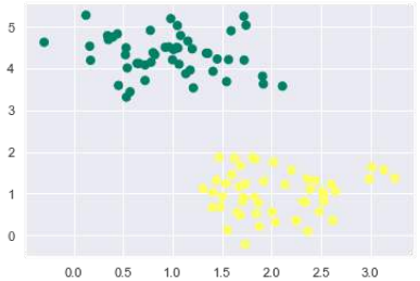
接下来,我们从 sklearn.datasets.samples_generator 创建一个样本数据集,其中包含线性可分离的数据,用于使用 SVM 进行分类:
from sklearn.datasets import make_blobs # 修正了导入路径,旧版本可能在 samples_generator

X, y = make_blobs(n_samples=100, centers=2,
                  random_state=0, cluster_std=0.50)
plt.scatter(X[:, 0], X[:, 1], c=y, s=50, cmap='summer')
plt.show() # 添加这一行以显示图形
生成包含 100 个样本和 2 个簇的样本数据集后,输出将如下所示。
我们知道 SVM 支持判别分类。它通过简单地在二维情况下找到一条线或在多维情况下找到一个流形来相互划分类别。它在上述数据集上实现如下:
xfit = np.linspace(-1, 3.5)
plt.scatter(X[:, 0], X[:, 1], c=y, s=50, cmap='summer')
plt.plot([0.6], [2.1], 'x', color='black', markeredgewidth=4, markersize=12) # 标记一个特定的点
for m, b in [(1, 0.65), (0.5, 1.6), (-0.2, 2.9)]:
    plt.plot(xfit, m * xfit + b, '-k') # 绘制多条可能的分类线
plt.xlim(-1, 3.5)
plt.show() # 添加这一行以显示图形
输出如下:
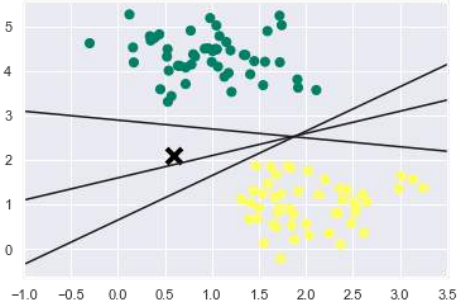
从上面的输出中我们可以看到,有三个不同的分离器可以完美地判别上述样本。
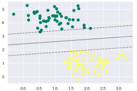
正如所讨论的,SVM 的主要目标是将数据集划分为类别以找到最大间隔超平面 (MMH),因此,我们不是在类别之间绘制一条零线,而是在每条线周围绘制一个到最近点的具有一定宽度的间隔。这可以这样做:
xfit = np.linspace(-1, 3.5)
plt.scatter(X[:, 0], X[:, 1], c=y, s=50, cmap='summer')
for m, b, d in [(1, 0.65, 0.33), (0.5, 1.6, 0.55), (-0.2, 2.9, 0.2)]:
    yfit = m * xfit + b
    plt.plot(xfit, yfit, '-k')
    plt.fill_between(xfit, yfit - d, yfit + d, edgecolor='none',
                     color='#AAAAAA', alpha=0.4) # 绘制间隔区域
plt.xlim(-1, 3.5)
plt.show() # 添加这一行以显示图形
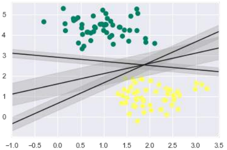
从输出中的上图中,我们可以很容易地观察到判别分类器中的“间隔”。SVM 将选择使间隔最大化的线。
接下来,我们将使用 Scikit-Learn 的支持向量分类器在此数据上训练 SVM 模型。在这里,我们使用线性核来拟合 SVM,如下所示:
from sklearn.svm import SVC # "Support vector classifier"
model = SVC(kernel='linear', C=1E10) # 修正为 SVC
model.fit(X, y)
输出如下:
SVC(C=10000000000.0, cache_size=200, class_weight=None, coef0=0.0,
    decision_function_shape='ovr', degree=3, gamma='auto',
    kernel='linear', max_iter=-1, probability=False, random_state=None,
    shrinking=True, tol=0.001, verbose=False) # gamma可能显示为'auto',取决于scikit-learn版本
现在,为了更好地理解,以下将绘制 2D SVC 的决策函数:
def plot_svc_decision_function(model, ax=None, plot_support=True): # 修正函数名
    if ax is None:
        ax = plt.gca()
    xlim = ax.get_xlim()
    ylim = ax.get_ylim()

    # 用于评估模型,我们需要创建网格,如下所示:
    x = np.linspace(xlim[0], xlim[1], 30)
    y = np.linspace(ylim[0], ylim[1], 30)
    Y, X_grid = np.meshgrid(y, x) # 修正为 X_grid
    xy = np.vstack([X_grid.ravel(), Y.ravel()]).T # 修正为 X_grid

    P = model.decision_function(xy).reshape(X_grid.shape) # 修正为 X_grid

    # 接下来,我们需要绘制决策边界和间隔,如下所示:
    ax.contour(X_grid, Y, P, colors='k',
               levels=[-1, 0, 1], alpha=0.5,
               linestyles=['--', '-', '--'])

    # 现在,类似地绘制支持向量,如下所示:
    if plot_support:
        ax.scatter(model.support_vectors_[:, 0],
                   model.support_vectors_[:, 1],
                   s=300, linewidth=1, facecolors='none');
    ax.set_xlim(xlim)
    ax.set_ylim(ylim)
现在,使用此函数来拟合我们的模型,如下所示:
plt.scatter(X[:, 0], X[:, 1], c=y, s=50, cmap='summer')
plot_svc_decision_function(model) # 调用修正后的函数名
plt.show() # 添加这一行以显示图形
从上面的输出中我们可以观察到,SVM 分类器拟合数据时带有间隔(即虚线)和支持向量,这些是拟合的关键元素,接触虚线。这些支持向量点存储在分类器的 support_vectors_ 属性中,如下所示:
model.support_vectors_
输出如下:
array([[0.5323772 , 3.31338909],
       [2.11114739, 3.57660449],
       [1.46870582, 1.86947425]])
SVM 核函数 (SVM Kernels)
在实践中,SVM 算法使用核函数来实现,核函数将输入数据空间转换为所需的形式。SVM 使用一种称为核技巧的技术,其中核函数接收低维输入空间并将其转换为高维空间。简单来说,核函数通过增加更多维度将不可分离的问题转换为可分离的问题。这使得 SVM 更加强大、灵活和准确。以下是 SVM 使用的一些核函数类型:
线性核 (Linear Kernel)
它可以用作任意两个观测值之间的点积。线性核的公式如下:
![]()
从上面的公式中,我们可以看到两个向量(例如 mathbfx 和 mathbfx_i)之间的乘积是每对输入值乘积的总和。
多项式核 (Polynomial Kernel)
它是线性核的更广义形式,并区分曲线或非线性输入空间。以下是多项式核的公式:
![]()
其中 d 是多项式的次数,我们需要在学习算法中手动指定。
径向基函数 (Radial Basis Function, RBF) 核
RBF 核主要用于 SVM 分类,将输入空间映射到无限维空间。以下公式从数学上解释了它:
![]()
其中 gamma 范围从 0 到 1。我们需要在学习算法中手动指定它。gamma 的一个好的默认值是 0.1。
正如我们为线性可分离数据实现了 SVM 一样,我们也可以在 Python 中为非线性可分离数据实现它。这可以通过使用核函数来完成。
示例
以下是使用核函数创建 SVM 分类器的示例。我们将使用 scikit-learn 中的鸢尾花数据集:
我们将从导入以下包开始:
import pandas as pd # 未直接使用,但通常用于数据处理
import numpy as np
from sklearn import svm, datasets
import matplotlib.pyplot as plt
现在,我们需要加载输入数据:
iris = datasets.load_iris()
从这个数据集中,我们取前两个特征,如下所示:
X = iris.data[:, :2]
y = iris.target
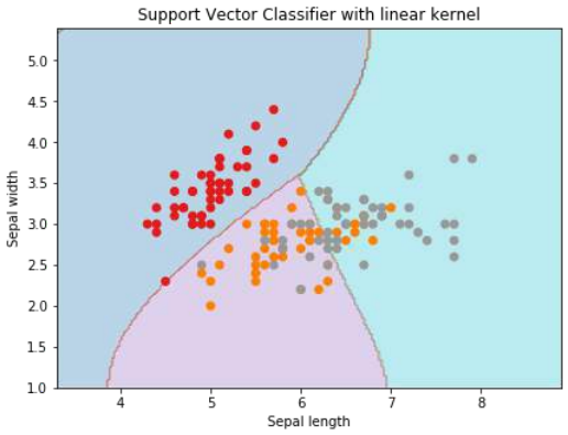
接下来,我们将绘制带有原始数据的 SVM 边界,如下所示:
x_min, x_max = X[:, 0].min() - 1, X[:, 0].max() + 1
y_min, y_max = X[:, 1].min() - 1, X[:, 1].max() + 1
h = (x_max / x_min)/100 # 这个 h 的计算可能不是最佳的,可能会导致网格点分布不均匀或过密。通常直接取一个小的固定步长。
# 修正 h 的计算方式
h = 0.02 # 使用一个小的固定步长

xx, yy = np.meshgrid(np.arange(x_min, x_max, h),
                     np.arange(y_min, y_max, h))
X_plot = np.c_[xx.ravel(), yy.ravel()]
现在,我们需要提供正则化参数的值,如下所示:
C = 1.0
接下来,可以创建 SVM 分类器对象,如下所示:
svc_classifier = svm.SVC(kernel='linear', C=C).fit(X, y) # 修正变量名 Svc_classifier
Z = svc_classifier.predict(X_plot)
Z = Z.reshape(xx.shape)

plt.figure(figsize=(15, 5))
plt.subplot(121)
plt.contourf(xx, yy, Z, cmap=plt.cm.tab10, alpha=0.3) # 修正 cmap,tab10 是正确的
plt.scatter(X[:, 0], X[:, 1], c=y, cmap=plt.cm.Set1) # 修正 cmap,Set1 是一个好选择
plt.xlabel('Sepal length')
plt.ylabel('Sepal width')
plt.xlim(xx.min(), xx.max())
plt.title('Support Vector Classifier with linear kernel')
plt.show() # 添加这一行以显示图形
输出
Text(0.5, 1.0, 'Support Vector Classifier with linear kernel')
为了使用 rbf 核创建 SVM 分类器,我们可以将核更改为 rbf,如下所示:
svc_classifier = svm.SVC(kernel='rbf', gamma='auto', C=C).fit(X, y) # 修正变量名 Svc_classifier,gamma='auto'
Z = svc_classifier.predict(X_plot)
Z = Z.reshape(xx.shape)

plt.figure(figsize=(15, 5))
plt.subplot(121)
plt.contourf(xx, yy, Z, cmap=plt.cm.tab10, alpha=0.3)
plt.scatter(X[:, 0], X[:, 1], c=y, cmap=plt.cm.Set1)
plt.xlabel('Sepal length')
plt.ylabel('Sepal width')
plt.xlim(xx.min(), xx.max())
plt.title('Support Vector Classifier with rbf kernel')
plt.show() # 添加这一行以显示图形
输出
Text(0.5, 1.0, 'Support Vector Classifier with rbf kernel')
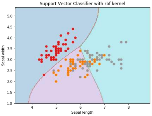
我们将 gamma 的值设为“auto”,但您也可以在 0 到 1 之间提供其值。
SVM 分类器的优缺点
SVM 分类器的优点
SVM 分类器提供高精度,并且在高维空间中表现良好。SVM 分类器基本上使用训练点的一个子集,因此最终使用的内存非常少。
SVM 分类器的缺点
它们的训练时间长,因此在实践中不适用于大型数据集。另一个缺点是 SVM 分类器在类重叠时表现不佳。
11. Classification Algorithms – Support Machine
Vector
Learning Machine with Python
(SVM)
Introduction to SVM
Support vector machines (SVMs) are powerful yet flexible supervised machine learning
algorithms which are used both for classification and regression. But generally, they are
used in classification problems. In 1960s, SVMs were first introduced but later they got
refined in 1990. SVMs have their unique way of implementation as compared to other
machine learning algorithms. Lately, they are extremely popular because of their ability
to handle multiple continuous and categorical variables.
Working of SVM
An SVM model is basically a representation of different classes in a hyperplane in
multidimensional space. The hyperplane will be generated in an iterative manner by SVM
so that the error can be minimized. The goal of SVM is to divide the datasets into classes
to find a maximum marginal hyperplane (MMH).
Y-Axis
Margin
Class A
Class B
Support
Vectors
X-Axis
The followings are important concepts in SVM:
Support Vectors: Datapoints that are closest to the hyperplane is called support
vectors. Separating line will be defined with the help of these data points.
Hyperplane: As we can see in the above diagram, it is a decision plane or space
which is divided between a set of objects having different classes.
Margin: It may be defined as the gap between two lines on the closet data points
of different classes. It can be calculated as the perpendicular distance from the line
to the support vectors. Large margin is considered as a good margin and small
margin is considered as a bad margin.
71
Machine Learning with Python
The main goal of SVM is to divide the datasets into classes to find a maximum marginal
hyperplane (MMH) and it can be done in the following two steps:
First, SVM will generate hyperplanes iteratively that segregates the classes in best
way.
Then, it will choose the hyperplane that separates the classes correctly.
Implementing SVM in Python
For implementing SVM in Python we will start with the standard libraries import as follows:
import numpy as np
import matplotlib.pyplot as plt
from scipy import stats
import seaborn as sns; sns.set()
Next, we are creating a sample dataset, having linearly separable data, from
sklearn.dataset.sample_generator for classification using SVM:
from sklearn.datasets.samples_generator import make_blobs
X, y = make_blobs(n_samples=100, centers=2,
random_state=0, cluster_std=0.50)
plt.scatter(X[:, 0], X[:, 1], c=y, s=50, cmap='summer');
The following would be the output after generating sample dataset having 100 samples
and 2 clusters:
We know that SVM supports discriminative classification. it divides the classes from each
other by simply finding a line in case of two dimensions or manifold in case of multiple
dimensions. It is implemented on the above dataset as follows:
xfit = np.linspace(-1, 3.5)
plt.scatter(X[:, 0], X[:, 1], c=y, s=50, cmap='summer')
72
Machine Learning with Python
plt.plot([0.6], [2.1], 'x', color='black', markeredgewidth=4, markersize=12)
for m, b in [(1, 0.65), (0.5, 1.6), (-0.2, 2.9)]:
plt.plot(xfit, m * xfit + b, '-k')
plt.xlim(-1, 3.5);
The output is as follows:
We can see from the above output that there are three different separators that perfectly
discriminate the above samples.
As discussed, the main goal of SVM is to divide the datasets into classes to find a maximum
marginal hyperplane (MMH) hence rather than drawing a zero line between classes we can
draw around each line a margin of some width up to the nearest point. It can be done as
follows:
xfit = np.linspace(-1, 3.5)
plt.scatter(X[:, 0], X[:, 1], c=y, s=50, cmap='summer')
for m, b, d in [(1, 0.65, 0.33), (0.5, 1.6, 0.55), (-0.2, 2.9, 0.2)]:
yfit = m * xfit + b
plt.plot(xfit, yfit, '-k')
plt.fill_between(xfit, yfit - d, yfit + d, edgecolor='none',
color='#AAAAAA', alpha=0.4)
plt.xlim(-1, 3.5);
73
Machine Learning with Python
From the above image in output, we can easily observe the “margins” within the
discriminative classifiers. SVM will choose the line that maximizes the margin.
Next, we will use Scikit-Learn’s support vector classifier to train an SVM model on this
data. Here, we are using linear kernel to fit SVM as follows:
from sklearn.svm import SVC # "Support vector classifier"
model = SVC(kernel='linear', C=1E10)
model.fit(X, y)
The output is as follows:
SVC(C=10000000000.0, cache_size=200, class_weight=None, coef0=0.0,
decision_function_shape='ovr', degree=3, gamma='auto_deprecated',
kernel='linear', max_iter=-1, probability=False, random_state=None,
shrinking=True, tol=0.001, verbose=False)
Now, for a better understanding, the following will plot the decision functions for 2D SVC:
def decision_function(model, ax=None, plot_support=True):
if ax is None:
ax = plt.gca()
xlim = ax.get_xlim()
ylim = ax.get_ylim()
For evaluating model, we need to create grid as follows:
x = np.linspace(xlim[0], xlim[1], 30)
y = np.linspace(ylim[0], ylim[1], 30)
74
Machine Learning with Python
Y, X = np.meshgrid(y, x)
xy = np.vstack([X.ravel(), Y.ravel()]).T
P = model.decision_function(xy).reshape(X.shape)
Next, we need to plot decision boundaries and margins as follows:
ax.contour(X, Y, P, colors='k',
levels=[-1, 0, 1], alpha=0.5,
linestyles=['--', '-', '--'])
Now, similarly plot the support vectors as follows:
if plot_support:
ax.scatter(model.support_vectors_[:, 0],
model.support_vectors_[:, 1],
s=300, linewidth=1, facecolors='none');
ax.set_xlim(xlim)
ax.set_ylim(ylim)
Now, use this function to fit our models as follows:
plt.scatter(X[:, 0], X[:, 1], c=y, s=50, cmap='summer')
decision_function(model);
75
Machine Learning with Python
We can observe from the above output that an SVM classifier fit to the data with margins
i.e. dashed lines and support vectors, the pivotal elements of this fit, touching the dashed
line. These support vector points are stored in the support_vectors_ attribute of the
classifier as follows:
model.support_vectors_
The output is as follows:
array([[0.5323772 , 3.31338909],
[2.11114739, 3.57660449],
[1.46870582, 1.86947425]])
SVM Kernels
In practice, SVM algorithm is implemented with kernel that transforms an input data space
into the required form. SVM uses a technique called the kernel trick in which kernel takes
a low dimensional input space and transforms it into a higher dimensional space. In simple
words, kernel converts non-separable problems into separable problems by adding more
dimensions to it. It makes SVM more powerful, flexible and accurate. The following are
some of the types of kernels used by SVM:
Linear Kernel
It can be used as a dot product between any two observations. The formula of linear kernel
is as below:
K(x, xi ) = sum(x ∗ xi )
From the above formula, we can see that the product between two vectors say x & x i is the
sum of the multiplication of each pair of input values.
Polynomial Kernel
It is more generalized form of linear kernel and distinguish curved or nonlinear input space.
Following is the formula for polynomial kernel:
K(x, xi) = 1 + sum(x * xi)^d
Here d is the degree of polynomial, which we need to specify manually in the learning
algorithm.
Radial Basis Function (RBF) Kernel
RBF kernel, mostly used in SVM classification, maps input space in indefinite dimensional
space. Following formula explains it mathematically:
K(x,xi) = exp(-gamma * sum((x – xi^2))
76
Machine Learning with Python
Here, gamma ranges from 0 to 1. We need to manually specify it in the learning algorithm.
A good default value of gamma is 0.1.
As we implemented SVM for linearly separable data, we can implement it in Python for the
data that is not linearly separable. It can be done by using kernels.
Example
The following is an example for creating an SVM classifier by using kernels. We will be
using iris dataset from scikit-learn:
We will start by importing following packages:
import pandas as pd
import numpy as np
from sklearn import svm, datasets
import matplotlib.pyplot as plt
Now, we need to load the input data:
iris = datasets.load_iris()
From this dataset, we are taking first two features as follows:
X = iris.data[:, :2]
y = iris.target
Next, we will plot the SVM boundaries with original data as follows:
x_min, x_max = X[:, 0].min() - 1, X[:, 0].max() + 1
y_min, y_max = X[:, 1].min() - 1, X[:, 1].max() + 1
h = (x_max / x_min)/100
xx, yy = np.meshgrid(np.arange(x_min, x_max, h),
np.arange(y_min, y_max, h))
X_plot = np.c_[xx.ravel(), yy.ravel()]
Now, we need to provide the value of regularization parameter as follows:
C = 1.0
Next, SVM classifier object can be created as follows:
Svc_classifier = svm.SVC(kernel='linear', C=C).fit(X, y)
Z = svc_classifier.predict(X_plot)
Z = Z.reshape(xx.shape)
plt.figure(figsize=(15, 5))
plt.subplot(121)
77
Machine Learning with Python
plt.contourf(xx, yy, Z, cmap=plt.cm.tab10, alpha=0.3)
plt.scatter(X[:, 0], X[:, 1], c=y, cmap=plt.cm.Set1)
plt.xlabel('Sepal length')
plt.ylabel('Sepal width')
plt.xlim(xx.min(), xx.max())
plt.title('Support Vector Classifier with linear kernel')
Output
Text(0.5, 1.0, 'Support Vector Classifier with linear kernel')
For creating SVM classifier with rbf kernel, we can change the kernel to rbf as follows:
Svc_classifier = svm.SVC(kernel='rbf', gamma =‘auto’,C=C).fit(X, y)
Z = svc_classifier.predict(X_plot)
Z = Z.reshape(xx.shape)
plt.figure(figsize=(15, 5))
plt.subplot(121)
plt.contourf(xx, yy, Z, cmap=plt.cm.tab10, alpha=0.3)
plt.scatter(X[:, 0], X[:, 1], c=y, cmap=plt.cm.Set1)
plt.xlabel('Sepal length')
plt.ylabel('Sepal width')
plt.xlim(xx.min(), xx.max())
plt.title('Support Vector Classifier with rbf kernel')
78
Machine Learning with Python
Output
Text(0.5, 1.0, 'Support Vector Classifier with rbf kernel')
We put the value of gamma to ‘auto’ but you can provide its value between 0 to 1 also.
Pros and Cons of SVM Classifiers
Pros of SVM classifiers
SVM classifiers offers great accuracy and work well with high dimensional space. SVM
classifiers basically use a subset of training points hence in result uses very less memory.
Cons of SVM classifiers
They have high training time hence in practice not suitable for large datasets. Another
disadvantage is that SVM classifiers do not work well with overlapping classes.