Python 机器学习
决策树简介
通常,决策树分析是一种可应用于许多领域的预测建模工具。决策树可以通过算法方法构建,该方法可以根据不同的条件以不同的方式分割数据集。决策树是属于监督算法类别中最强大的算法。
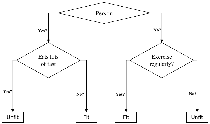
它们既可用于分类任务,也可用于回归任务。树的两个主要实体是决策节点(数据在此处分割)和叶子(我们得到结果)。下面给出了一个二叉树的示例,用于根据年龄、饮食习惯和运动习惯等各种信息预测一个人是否健康:
人
年龄 > 30 吗?
- 是?
- 吃很多快餐吗?
- 是? -> 不健康
- 否? -> 健康
- 吃很多快餐吗?
- 否?
- 经常锻炼吗?
- 是? -> 健康
- 否? -> 不健康
- 经常锻炼吗?
在上述决策树中,问题是决策节点,最终结果是叶子。我们有以下两种类型的决策树:
- 分类决策树:在这种决策树中,决策变量是分类的。上述决策树就是分类决策树的一个例子。
- 回归决策树:在这种决策树中,决策变量是连续的。
实现决策树算法
基尼指数 (Gini Index)
它是用于评估数据集中二元分割的成本函数的名称,并与分类目标变量“成功”或“失败”一起使用。
基尼指数值越高,同质性越高。完美的基尼指数值为 0,最差为 0.5(对于 2 类问题)。分割的基尼指数可以通过以下步骤计算:
- 首先,使用公式 计算子节点的基尼指数,这是成功和失败概率的平方和。
- 接下来,使用该分割中每个节点的加权基尼分数计算分割的基尼指数。
分类和回归树 (CART) 算法使用基尼方法生成二元分割。
分割创建 (Split Creation)
分割基本上包括数据集中的一个属性和一个值。我们可以在数据集的帮助下创建分割,分为以下三个部分:
- 第一部分:计算基尼分数:我们刚刚在上一节中讨论了这部分。
- 第二部分:分割数据集:它可定义为将数据集分离为两行列表,其中包含属性的索引和该属性的分割值。从数据集中获得两组(右和左)后,我们可以使用第一部分中计算的基尼分数计算分割值。分割值将决定属性将驻留在哪个组中。
- 第三部分:评估所有分割:在找到基尼分数并分割数据集之后,下一部分是评估所有分割。为此,首先,我们必须检查与每个属性关联的每个值作为候选分割。然后我们需要通过评估分割的成本来找到最佳可能的分割。最佳分割将用作决策树中的节点。
构建树 (Building a Tree)
众所周知,一棵树有根节点和叶节点。创建根节点后,我们可以通过以下两个部分构建树:
第一部分:叶节点创建 (Terminal node creation)
在创建决策树的叶节点时,一个重要点是决定何时停止生长树或创建进一步的叶节点。这可以通过使用两个标准来完成,即最大树深度和最小节点记录,如下所示:
- 最大树深度:顾名思义,这是树中根节点后的最大节点数。一旦树达到最大深度,即一旦树获得最大数量的叶节点,我们必须停止添加叶节点。
- 最小节点记录:它可定义为给定节点负责的最小训练模式数。一旦树达到这些最小节点记录或低于此最小值,我们必须停止添加叶节点。叶节点用于进行最终预测。
第二部分:递归分割 (Recursive Splitting)
正如我们了解了何时创建叶节点一样,现在我们可以开始构建我们的树。递归分割是一种构建树的方法。在这种方法中,一旦创建了一个节点,我们就可以通过一遍又一遍地调用相同的函数,在由分割数据集生成的每组数据上递归地创建子节点(添加到现有节点的节点)。
预测 (Prediction)
构建决策树后,我们需要对其进行预测。基本上,预测涉及使用专门提供的数据行导航决策树。
我们可以借助递归函数进行预测,如上所述。相同的预测例程会再次与左或右子节点一起调用。
假设 (Assumptions)
在创建决策树时,我们做出了以下一些假设:
- 在准备决策树时,训练集是根节点。
- 决策树分类器倾向于特征值为分类的。如果您想使用连续值,则必须在模型构建之前对其进行离散化。
- 根据属性的值,记录会递归地分布。
- 将使用统计方法将属性放置在任何节点位置,即作为根节点或内部节点。
在 Python 中实现
示例
在以下示例中,我们将在 Pima Indian Diabetes 数据集上实现决策树分类器:
首先,导入必要的 python 包:
import pandas as pd
from sklearn.tree import DecisionTreeClassifier
from sklearn.model_selection import train_test_split
接下来,从其网页链接下载鸢尾花数据集,如下所示:
col_names = ['pregnant', 'glucose', 'bp', 'skin', 'insulin', 'bmi', 'pedigree',
             'age', 'label']
pima = pd.read_csv(r"C:\pima-indians-diabetes.csv", header=None,
                   names=col_names)
pima.head()
输出:
   pregnant  glucose  bp  skin  insulin   bmi  pedigree  age  label
0         6      148  72    35        0  33.6     0.627   50      1
1         1       85  66    29        0  26.6     0.351   31      0
2         8      183  64     0        0  23.3     0.672   32      1
3         1       89  66    23       94  28.1     0.167   21      0
4         0      137  40    35      168  43.1     2.288   33      1
现在,将数据集分割为特征和目标变量,如下所示:
feature_cols = ['pregnant', 'insulin', 'bmi', 'age', 'glucose', 'bp', 'pedigree']
X = pima[feature_cols] # 特征
y = pima.label       # 目标变量
接下来,我们将数据划分为训练集和测试集。以下代码将把数据集分割为 70% 的训练数据和 30% 的测试数据:
X_train, X_test, y_train, y_test = train_test_split(X, y, test_size=0.3,
                                                    random_state=1)
接下来,借助 sklearn 的 DecisionTreeClassifier 类训练模型,如下所示:
clf = DecisionTreeClassifier()
clf = clf.fit(X_train, y_train)
最后,我们需要进行预测。这可以通过以下脚本完成:
y_pred = clf.predict(X_test)
接下来,我们可以获取准确率分数、混淆矩阵和分类报告,如下所示:
from sklearn.metrics import classification_report, confusion_matrix, accuracy_score

result = confusion_matrix(y_test, y_pred)
print("Confusion Matrix:")
print(result)

result1 = classification_report(y_test, y_pred)
print("Classification Report:")
print(result1)

result2 = accuracy_score(y_test, y_pred)
print("Accuracy:", result2)
输出
Confusion Matrix:
[[116  30]
 [ 46  39]]

Classification Report:
              precision    recall  f1-score   support

           0       0.72      0.79      0.75       146
           1       0.57      0.46      0.51        85

    accuracy                           0.67       231
   macro avg       0.64      0.63      0.63       231
weighted avg       0.66      0.67      0.66       231

Accuracy: 0.670995670995671
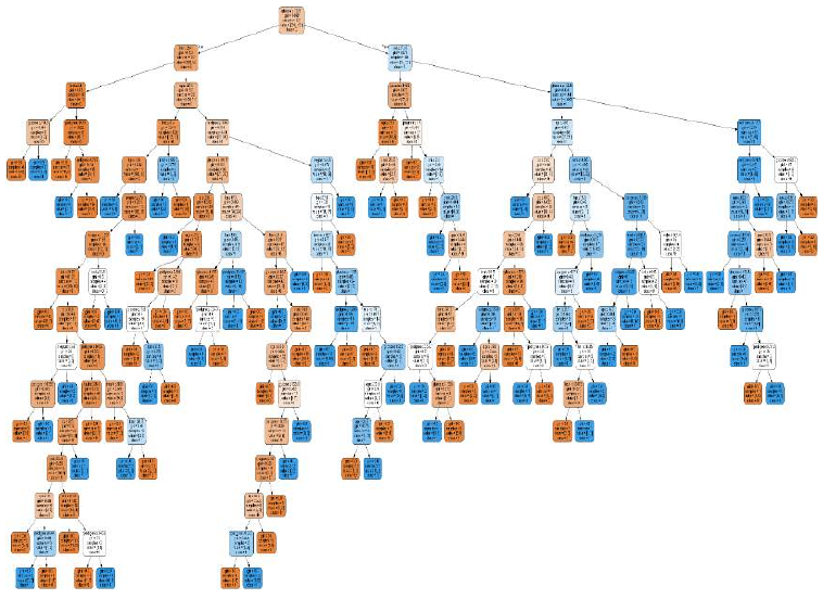
可视化决策树 (Visualizing Decision Tree)
上述决策树可以通过以下代码进行可视化:
from sklearn.tree import export_graphviz
# from sklearn.externals.six import StringIO # 此导入在较新版本中已被弃用,直接使用 io.StringIO
import io # 新增导入
from IPython.display import Image
import pydotplus

dot_data = io.StringIO() # 替换 StringIO

export_graphviz(clf, out_file=dot_data,
                filled=True, rounded=True,
                special_characters=True, feature_names=feature_cols,
                class_names=['0', '1']) # 修正 class_names 的数据类型,应为字符串

graph = pydotplus.graph_from_dot_data(dot_data.getvalue())
graph.write_png('Pima_diabetes_Tree.png')
Image(graph.create_png())
12. Classification Algorithms Machine
– Decision
Learning with Tree
Python
Introduction to Decision Tree
In general, Decision tree analysis is a predictive modelling tool that can be applied across
many areas. Decision trees can be constructed by an algorithmic approach that can split
the dataset in different ways based on different conditions. Decisions tress are the most
powerful algorithms that falls under the category of supervised algorithms.
They can be used for both classification and regression tasks. The two main entities of a
tree are decision nodes, where the data is split and leaves, where we got outcome. The
example of a binary tree for predicting whether a person is fit or unfit providing various
information like age, eating habits and exercise habits, is given below:
Yes?
Person
age>30?
No?
Yes?
Eats lots
of fast
food?
No?
Yes?
Exercise
regularly?
No?
Unfit
Fit
Fit
Unfit
In the above decision tree, the question are decision nodes and final outcomes are leaves.
We have the following two types of decision trees:
Classification decision trees: In this kind of decision trees, the decision variable
is categorical. The above decision tree is an example of classification decision tree.
Regression decision trees: In this kind of decision trees, the decision variable is
continuous.
80
Machine Learning with Python
Implementing Decision Tree Algorithm
Gini Index
It is the name of the cost function that is used to evaluate the binary splits in the dataset
and works with the categorial target variable “Success” or “Failure”.
Higher the value of Gini index, higher the homogeneity. A perfect Gini index value is 0 and
worst is 0.5 (for 2 class problem). Gini index for a split can be calculated with the help of
following steps:
First, calculate Gini index for sub-nodes by using the formula p^2+q^2 , which is
the sum of the square of probability for success and failure.
Next, calculate Gini index for split using weighted Gini score of each node of that
split.
Classification and Regression Tree (CART) algorithm uses Gini method to generate binary
splits.
Split Creation
A split is basically including an attribute in the dataset and a value. We can create a split
in dataset with the help of following three parts:
Part1: Calculating Gini Score: We have just discussed this part in the previous
section.
Part2: Splitting a dataset: It may be defined as separating a dataset into two
lists of rows having index of an attribute and a split value of that attribute. After
getting the two groups - right and left, from the dataset, we can calculate the value
of split by using Gini score calculated in first part. Split value will decide in which
group the attribute will reside.
Part3: Evaluating all splits: Next part after finding Gini score and splitting
dataset is the evaluation of all splits. For this purpose, first, we must check every
value associated with each attribute as a candidate split. Then we need to find the
best possible split by evaluating the cost of the split. The best split will be used as
a node in the decision tree.
Building a Tree
As we know that a tree has root node and terminal nodes. After creating the root node,
we can build the tree by following two parts:
Part1: Terminal node creation
While creating terminal nodes of decision tree, one important point is to decide when to
stop growing tree or creating further terminal nodes. It can be done by using two criteria
namely maximum tree depth and minimum node records as follows:
Maximum Tree Depth: As name suggests, this is the maximum number of the
nodes in a tree after root node. We must stop adding terminal nodes once a tree
81
Machine Learning with Python
reached at maximum depth i.e. once a tree got maximum number of terminal
nodes.
Minimum Node Records: It may be defined as the minimum number of training
patterns that a given node is responsible for. We must stop adding terminal nodes
once tree reached at these minimum node records or below this minimum.
Terminal node is used to make a final prediction.
Part2: Recursive Splitting
As we understood about when to create terminal nodes, now we can start building our
tree. Recursive splitting is a method to build the tree. In this method, once a node is
created, we can create the child nodes (nodes added to an existing node) recursively on
each group of data, generated by splitting the dataset, by calling the same function again
and again.
Prediction
After building a decision tree, we need to make a prediction about it. Basically, prediction
involves navigating the decision tree with the specifically provided row of data.
We can make a prediction with the help of recursive function, as did above. The same
prediction routine is called again with the left or the child right nodes.
Assumptions
The following are some of the assumptions we make while creating decision tree:
While preparing decision trees, the training set is as root node.
Decision tree classifier prefers the features values to be categorical. In case if you
want to use continuous values then they must be done discretized prior to model
building.
Based on the attribute’s values, the records are recursively distributed.
Statistical approach will be used to place attributes at any node position i.e.as root
node or internal node.
Implementation in Python
Example
In the following example, we are going to implement Decision Tree classifier on Pima
Indian Diabetes:
First, start with importing necessary python packages:
import pandas as pd
from sklearn.tree import DecisionTreeClassifier
from sklearn.model_selection import train_test_split
82
Machine Learning with Python
Next, download the iris dataset from its weblink as follows:
col_names = ['pregnant', 'glucose', 'bp', 'skin', 'insulin', 'bmi', 'pedigree',
'age', 'label']
pima = pd.read_csv(r"C:\pima-indians-diabetes.csv", header=None,
names=col_names)
pima.head()
pregnant
glucose
bp
skin
insulin
bmi
pedigree
age
label
0
6
148
72
35
0
33.6
0.627
50
1
1
1
85
66
29
0
26.6
0.351
31
0
2
8
183
64
0
0
23.3
0.672
32
1
3
1
89
66
23
94
28.1
0.167
21
0
4
0
137
40
35
168
43.1
2.288
33
1
Now, split the dataset into features and target variable as follows:
feature_cols = ['pregnant', 'insulin', 'bmi', 'age','glucose','bp','pedigree']
X = pima[feature_cols] # Features
y = pima.label # Target variable
Next, we will divide the data into train and test split. The following code will split the
dataset into 70% training data and 30% of testing data:
X_train, X_test, y_train, y_test = train_test_split(X, y, test_size=0.3,
random_state=1)
Next, train the model with the help of DecisionTreeClassifier class of sklearn as
follows:
clf = DecisionTreeClassifier()
clf = clf.fit(X_train,y_train)
At last we need to make prediction. It can be done with the help of following script:
y_pred = clf.predict(X_test)
Next, we can get the accuracy score, confusion matrix and classification report as follows:
from sklearn.metrics import classification_report, confusion_matrix,
accuracy_score
result = confusion_matrix(y_test, y_pred)
print("Confusion Matrix:")
print(result)
result1 = classification_report(y_test, y_pred)
print("Classification Report:",)
print (result1)
83
Machine Learning with Python
result2 = accuracy_score(y_test,y_pred)
print("Accuracy:",result2)
Output
Confusion Matrix:
[[116
30]
[ 46
39]]
Classification Report:
precision
recall
f1-score
support
0
0.72
0.79
0.75
146
1
0.57
0.46
0.51
85
micro avg
0.67
0.67
0.67
231
macro avg
0.64
0.63
0.63
231
weighted avg
0.66
0.67
0.66
231
Accuracy: 0.670995670995671
Visualizing Decision Tree
The above decision tree can be visualized with the help of following code:
from sklearn.tree import export_graphviz
from sklearn.externals.six import StringIO
from IPython.display import Image
import pydotplus
dot_data = StringIO()
export_graphviz(clf, out_file=dot_data,
filled=True, rounded=True,
special_characters=True,feature_names =
feature_cols,class_names=['0','1'])
graph = pydotplus.graph_from_dot_data(dot_data.getvalue())
graph.write_png('Pima_diabetes_Tree.png')
Image(graph.create_png())