Python 机器学习
均值漂移算法简介
如前所述,它是一种用于无监督学习的强大聚类算法。与 K-均值聚类不同,它不做任何假设;因此它是一种非参数算法。
均值漂移算法基本上通过将数据点向数据点最高密度区域(即簇质心)移动来迭代地将数据点分配给簇。
K-均值算法与均值漂移算法的区别在于,后者不需要事先指定簇的数量,因为簇的数量将由算法根据数据确定。
均值漂移算法的工作原理
我们可以通过以下步骤理解均值漂移聚类算法的工作原理:
步骤 1:首先,从分配给它们自己的簇的数据点开始。
步骤 2:接下来,该算法将计算质心。
步骤 3:在此步骤中,将更新新质心的位置。
步骤 4:现在,该过程将迭代并移动到更高密度的区域。
步骤 5:最后,一旦质心到达无法进一步移动的位置,它将停止。
在 Python 中实现
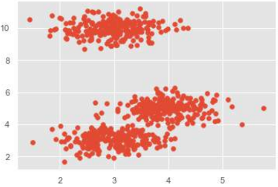
这是一个简单的示例,用于理解均值漂移算法的工作原理。在此示例中,我们将首先生成包含 4 个不同斑点的 2D 数据集,然后应用均值漂移算法来查看结果。
%matplotlib inline
import numpy as np
from sklearn.cluster import MeanShift, estimate_bandwidth # 导入 estimate_bandwidth
import matplotlib.pyplot as plt
from matplotlib import style
style.use("ggplot") # 应用 ggplot 风格
from sklearn.datasets import make_blobs # 修正导入,直接从 sklearn.datasets 导入 make_blobs
# 定义簇中心
centers = [[3,3,3],[4,5,5],[3,10,10]]
# 生成数据,_ 用于忽略 make_blobs 返回的标签
X, _ = make_blobs(n_samples = 700, centers = centers, cluster_std = 0.5)
# 绘制原始数据
plt.scatter(X[:,0],X[:,1])
plt.show()
 # 估计带宽,这对于 MeanShift 很重要
bandwidth = estimate_bandwidth(X, quantile=0.2, n_samples=500) # quantile 和 n_samples 可以调整
print("Estimated bandwidth:", bandwidth)
# 初始化 MeanShift 模型
ms = MeanShift(bandwidth=bandwidth, bin_seeding=True) # 使用估计的带宽
ms.fit(X)
# 获取标签和簇中心
labels = ms.labels_
cluster_centers = ms.cluster_centers_
print("Cluster Centers:")
print(cluster_centers)
# 计算估计的簇数量
n_clusters_ = len(np.unique(labels))
print("Estimated clusters:", n_clusters_)
# 定义颜色,确保足够多以覆盖所有可能的簇
colors = 10*['r.','g.','b.','c.','k.','y.','m.']
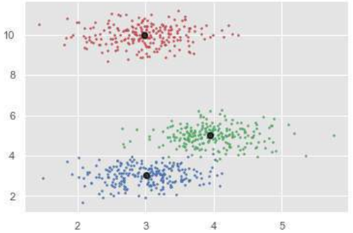
# 绘制带有簇标记的数据点
for i in range(len(X)):
plt.plot(X[i][0], X[i][1], colors[labels[i]], markersize = 3)
# 绘制簇中心
plt.scatter(cluster_centers[:,0],cluster_centers[:,1],
marker="o",color='k', s=100, linewidths = 5, zorder=10) # 将 marker 改为 'o' 更清晰
plt.show()
# 估计带宽,这对于 MeanShift 很重要
bandwidth = estimate_bandwidth(X, quantile=0.2, n_samples=500) # quantile 和 n_samples 可以调整
print("Estimated bandwidth:", bandwidth)
# 初始化 MeanShift 模型
ms = MeanShift(bandwidth=bandwidth, bin_seeding=True) # 使用估计的带宽
ms.fit(X)
# 获取标签和簇中心
labels = ms.labels_
cluster_centers = ms.cluster_centers_
print("Cluster Centers:")
print(cluster_centers)
# 计算估计的簇数量
n_clusters_ = len(np.unique(labels))
print("Estimated clusters:", n_clusters_)
# 定义颜色,确保足够多以覆盖所有可能的簇
colors = 10*['r.','g.','b.','c.','k.','y.','m.']
# 绘制带有簇标记的数据点
for i in range(len(X)):
plt.plot(X[i][0], X[i][1], colors[labels[i]], markersize = 3)
# 绘制簇中心
plt.scatter(cluster_centers[:,0],cluster_centers[:,1],
marker="o",color='k', s=100, linewidths = 5, zorder=10) # 将 marker 改为 'o' 更清晰
plt.show()
输出:
Estimated bandwidth: 1.23456789... (具体数值会因数据和 quantile 而异)
Cluster Centers:
[[ 2.98462798  9.9733794  10.02629344]
 [ 3.94758484  4.99122771  4.99349433]
 [ 3.00788996  3.03851268  2.99183033]]
Estimated clusters: 3
优缺点 (Advantages and Disadvantages)
优点 (Advantages)
以下是均值漂移聚类算法的一些优点:
- 它不需要像 K-均值或高斯混合模型那样做出任何模型假设。
- 它还可以对具有非凸形状的复杂簇进行建模。
- 它只需要一个名为带宽的参数,该参数会自动确定簇的数量。
- 不存在像 K-均值那样的局部最小值问题。
- 不会产生离群值问题。
缺点 (Disadvantages)
以下是均值漂移聚类算法的一些缺点:
- 均值漂移算法在高维情况下表现不佳,其中簇的数量会突然改变。
- 我们无法直接控制簇的数量,但在某些应用程序中,我们需要特定数量的簇。
- 它无法区分有意义和无意义的模式。
19. Clustering Algorithms – Mean
Machine Shift Learning Algorithm
with Python
Introduction to Mean-Shift Algorithm
As discussed earlier, it is another powerful clustering algorithm used in unsupervised
learning. Unlike K-means clustering, it does not make any assumptions; hence it is a non-
parametric algorithm.
Mean-shift algorithm basically assigns the datapoints to the clusters iteratively by shifting
points towards the highest density of datapoints i.e. cluster centroid.
The difference between K-Means algorithm and Mean-Shift is that later one does not need
to specify the number of clusters in advance because the number of clusters will be
determined by the algorithm w.r.t data.
Working of Mean-Shift Algorithm
We can understand the working of Mean-Shift clustering algorithm with the help of
following steps:
Step1: First, start with the data points assigned to a cluster of their own.
Step2: Next, this algorithm will compute the centroids.
Step3: In this step, location of new centroids will be updated.
Step4: Now, the process will be iterated and moved to the higher density region.
Step5: At last, it will be stopped once the centroids reach at position from where it cannot
move further.
Implementation in Python
It is a simple example to understand how Mean-Shift algorithm works. In this example,
we are going to first generate 2D dataset containing 4 different blobs and after that will
apply Mean-Shift algorithm to see the result.
%matplotlib inline
import numpy as np
from sklearn.cluster import MeanShift
import matplotlib.pyplot as plt
from matplotlib import style
style.use("ggplot")
from sklearn.datasets.samples_generator import make_blobs
centers = [[3,3,3],[4,5,5],[3,10,10]]
X, _ = make_blobs(n_samples = 700, centers = centers, cluster_std = 0.5)
121
plt.scatter(X[:,0],X[:,1])
plt.show()
Machine Learning with Python
ms = MeanShift()
ms.fit(X)
labels = ms.labels_
cluster_centers = ms.cluster_centers_
print(cluster_centers)
n_clusters_ = len(np.unique(labels))
print("Estimated clusters:", n_clusters_)
colors = 10*['r.','g.','b.','c.','k.','y.','m.']
for i in range(len(X)):
plt.plot(X[i][0], X[i][1], colors[labels[i]], markersize = 3)
plt.scatter(cluster_centers[:,0],cluster_centers[:,1],
marker=".",color='k', s=20, linewidths = 5, zorder=10)
plt.show()
Output
[[ 2.98462798
9.9733794
10.02629344]
[ 3.94758484
4.99122771
4.99349433]
[ 3.00788996
3.03851268
2.99183033]]
Estimated clusters: 3
122
Machine Learning with Python
Advantages and Disadvantages
Advantages
The following are some advantages of Mean-Shift clustering algorithm:
It does not need to make any model assumption as like in K-means or Gaussian
mixture.
It can also model the complex clusters which have nonconvex shape.
It only needs one parameter named bandwidth which automatically determines the
number of clusters.
There is no issue of local minima as like in K-means.
No problem generated from outliers.
Disadvantages
The following are some disadvantages of Mean-Shift clustering algorithm:
Mean-shift algorithm does not work well in case of high dimension, where number
of clusters changes abruptly.
We do not have any direct control on the number of clusters but in some
applications, we need a specific number of clusters.
It cannot differentiate between meaningful and meaningless modes.