机器学习Python教程
引言
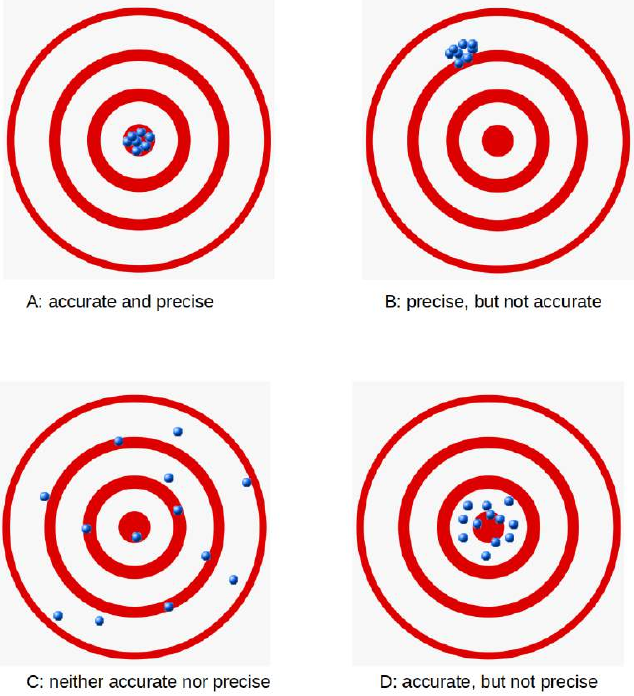
 无论是在机器学习中,还是在日常生活中,尤其是在商业领域,你都会听到诸如“你的产品有多准确?”或“你的机器有多精密?”之类的问题。当人们听到“这是该领域最准确的产品!”或“这台机器具有最高的精密性!”这样的回答时,他们会感到心安。难道不应该吗?事实上,“准确(accurate)”和“精密(precise)”这两个词经常互换使用。我们将在后面给出精确的定义,但简而言之,我们可以说:准确性衡量的是测量值与特定值之间的接近程度,而精密性则是衡量测量值彼此之间的接近程度。
这些术语在机器学习中也极其重要。我们需要它们来评估机器学习算法,或者更确切地说,是它们的结果。
在本章的 Python 机器学习教程中,我们将介绍四个重要的指标。这些指标用于评估分类结果。它们是:
-
准确率(Accuracy)
-
精确率(Precision)
-
召回率(Recall)
-
F1-分数(F1-Score)
我们将逐一介绍这些指标,并讨论它们的优缺点。每个指标都衡量分类器性能的不同方面。这些指标对于我们机器学习教程的所有章节都至关重要。
准确率(Accuracy)
准确性衡量的是测量值与特定值之间的接近程度,而精密性是衡量测量值彼此之间的接近程度,即不一定与特定值接近。换句话说:如果我们有一组对同一数量重复测量得到的数据点,如果它们的平均值接近被测量量的真实值,则称这组数据是准确的。另一方面,如果这些值彼此接近,则称这组数据是精密的。这两个概念是相互独立的,这意味着这组数据可以准确、或精密、或两者兼具、或两者都不是。我们通过以下图示来说明:
混淆矩阵(Confusion Matrix)
在我们继续讨论准确率这个术语之前,我们想确保你理解什么是混淆矩阵。
混淆矩阵,也称为列联表或误差矩阵,用于可视化分类器的性能。
矩阵的列表示预测类别的实例,而行表示实际类别的实例。(注意:这也可以反过来。)
在二元分类的情况下,该表有 2 行 2 列。
我们想通过一个例子来演示这个概念。
示例:
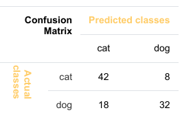
这意味着分类器正确预测了 42 个猫的实例,错误地将 8 个猫的实例预测为狗。它正确预测了 32 个狗的实例。有 18 个实例被错误地预测为猫而非狗。
分类中的准确率(Accuracy in Classification)
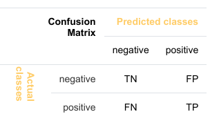
我们对机器学习感兴趣,准确率也用作统计度量。准确率是一种统计度量,定义为分类器做出的正确预测(真阳性(TP)和真阴性(TN))的数量除以分类器做出的所有预测的总和,包括假阳性(FP)和假阴性(FN)。因此,量化二元准确率的公式为:
其中:
-
(真阳性)
-
(假阳性)
-
(真阴性)
-
(假阴性)
相应的混淆矩阵如下所示:
现在我们将计算猫狗分类结果的准确率。这里我们看到的是“猫”和“狗”,而不是“真”和“假”。我们可以这样计算准确率:
TP=42
TN=32
FP=8
FN=18
Accuracy=(TP+TN)/(TP+TN+FP+FN)
Accuracy=(42+32)/(42+8+18+32)=74/100=0.74
print(Accuracy)
0.74
让我们假设我们有一个总是预测“狗”的分类器。
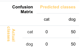
在这种情况下,我们的准确率为 0.5:
TP=0,TN=50,FP=50,FN=0
Accuracy=(TP+TN)/(TP+TN+FP+FN)
Accuracy=(0+50)/(0+50+50+0)=50/100=0.5
print(Accuracy)
0.5
准确率悖论(Accuracy Paradox)
我们将演示所谓的准确率悖论。
一个垃圾邮件识别分类器由以下混淆矩阵描述:
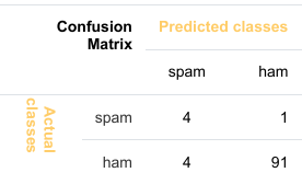
TP=4,TN=91,FP=1,FN=4
accuracy=(TP+TN)/(TP+TN+FP+FN)
accuracy=(4+91)/(4+91+1+4)=95/100=0.95
print(accuracy)
0.95
以下分类器仅预测“非垃圾邮件”,并且具有相同的准确率。
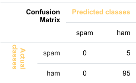
TP=0,TN=95,FP=5,FN=0
accuracy=(TP+TN)/(TP+TN+FP+FN)
accuracy=(0+95)/(0+95+5+0)=95/100=0.95
print(accuracy)
0.95
这个分类器的准确率是 95%,即使它完全无法识别任何垃圾邮件。
精确率(Precision)
精确率是正确识别的正例与所有预测为正例的比率,即正确和错误地预测为正例的情况。精确率是检索到的文档中与查询相关的文档所占的比例。公式为:
我们将通过一个例子来演示这一点。
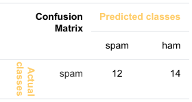 |
我们可以计算我们示例的精确率:
TP=114
FP=14
(FN(0) 和 TN(12) 在公式中不需要!)
precision=TP/(TP+FP)
precision=114/(114+14)=114/128≈0.89
print(f"precision: {precision:4.2f}")
precision: 0.89
思考: 在继续阅读之前,思考一下精确率的价值意味着什么。如果你看一下我们垃圾邮件过滤示例的精确率度量,它告诉你什么关于垃圾邮件过滤器的质量?一个理想的垃圾邮件过滤器的混淆矩阵结果是什么样子的?高 FP 或 FN 值哪个更糟糕?你会在下面的解释中间接找到答案。
顺便说一句,理想的垃圾邮件过滤器,其 FP 和 FN 值都为 0。
上述结果意味着每 100 封邮件中,有 11 封会被分类为非垃圾邮件,即使它们是垃圾邮件。89 封被正确分类为非垃圾邮件。这是我们应该讨论错误分类成本的地方。如果一封垃圾邮件没有被识别为“垃圾邮件”而是作为“非垃圾邮件”呈现给我们,这是很麻烦的。如果百分比不是太高,这很烦人但不是灾难。相反,如果一封非垃圾邮件被错误地标记为垃圾邮件,那么在许多情况下,这封邮件将不会显示,甚至会自动删除。例如,这会带来失去客户和朋友的高风险。精确率这个衡量标准没有说明最后提到的这类问题。其他衡量标准呢?
我们将看看召回率和 F1-分数。
召回率(Recall)
召回率,也称为灵敏度,是正确识别的正例与所有实际正例的比率,即“假阴性”和“真阳性”的总和。
TP=114
FN=0
(FP(14) 和 TN(12) 在公式中不需要!)
recall=TP/(TP+FN)
print(f"recall: {recall:4.2f}")
recall=114/(114+0)=1.00
值为 1 意味着没有非垃圾邮件被错误地标记为垃圾邮件。对于一个好的垃圾邮件过滤器来说,这个值应该为 1,这很重要。我们之前已经讨论过这一点。
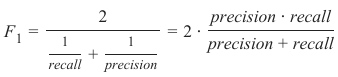
F1-分数 (F1-Score)
我们将要探讨的最后一个衡量指标是 F1-分数。
F1-分数是精确率 (Precision) 和召回率 (Recall) 的调和平均值,公式如下:
以下代码和表格展示了在不同误报 (FP) 和漏报 (FN) 值下,准确率、精确率、召回率和 F1-分数的表现。我们假设总样本数为 100,并且 真阴性 (TN) 值设为 5%,即 。因此,真阳性 (TP) 值可以通过 计算得出。
TN = 5 # 我们将真阴性值设置为 5%
print("  FN    FP    TP   pre   acc   rec    f1")
for FN in range(0, 7):
    for FP in range(0, FN + 1):
        # FN, FP, TN 和 TP 的总和为 100:
        TP = 100 - FN - FP - TN

        # 计算精确率
        precision = TP / (TP + FP)

        # 计算准确率
        accuracy = (TP + TN) / (TP + TN + FP + FN)

        # 计算召回率
        recall = TP / (TP + FN)

        # 计算 F1-分数
        f1_score = 2 * precision * recall / (precision + recall)

        print(f"{FN:6.2f}{FP:6.2f}{TP:6.2f}{precision:6.2f}{accuracy:6.2f}{recall:6.2f}{f1_score:6.2f}")
|
FN |
FP |
TP |
pre |
acc |
rec |
f1 |
|
0.00 |
0.00 |
95.00 |
1.00 |
1.00 |
1.00 |
1.00 |
|
1.00 |
0.00 |
94.00 |
1.00 |
0.99 |
0.99 |
0.99 |
|
1.00 |
1.00 |
93.00 |
0.99 |
0.99 |
0.99 |
0.99 |
|
2.00 |
0.00 |
93.00 |
1.00 |
0.98 |
0.98 |
0.99 |
|
2.00 |
1.00 |
92.00 |
0.99 |
0.98 |
0.98 |
0.98 |
|
2.00 |
2.00 |
91.00 |
0.98 |
0.98 |
0.98 |
0.98 |
|
3.00 |
0.00 |
92.00 |
1.00 |
0.97 |
0.97 |
0.98 |
|
3.00 |
1.00 |
91.00 |
0.99 |
0.97 |
0.97 |
0.98 |
|
3.00 |
2.00 |
90.00 |
0.98 |
0.97 |
0.97 |
0.97 |
|
3.00 |
3.00 |
89.00 |
0.97 |
0.97 |
0.97 |
0.97 |
|
4.00 |
0.00 |
91.00 |
1.00 |
0.96 |
0.96 |
0.98 |
|
4.00 |
1.00 |
90.00 |
0.99 |
0.96 |
0.96 |
0.97 |
|
4.00 |
2.00 |
89.00 |
0.98 |
0.96 |
0.96 |
0.97 |
|
4.00 |
3.00 |
88.00 |
0.97 |
0.96 |
0.96 |
0.96 |
|
4.00 |
4.00 |
87.00 |
0.96 |
0.96 |
0.96 |
0.96 |
|
5.00 |
0.00 |
90.00 |
1.00 |
0.95 |
0.95 |
0.97 |
|
5.00 |
1.00 |
89.00 |
0.99 |
0.95 |
0.95 |
0.97 |
|
5.00 |
2.00 |
88.00 |
0.98 |
0.95 |
0.95 |
0.96 |
|
5.00 |
3.00 |
87.00 |
0.97 |
0.95 |
0.94 |
0.96 |
|
5.00 |
4.00 |
86.00 |
0.95 |
0.95 |
0.94 |
0.95 |
|
5.00 |
5.00 |
85.00 |
0.94 |
0.95 |
0.94 |
0.94 |
|
6.00 |
0.00 |
89.00 |
1.00 |
0.94 |
0.94 |
0.97 |
|
6.00 |
1.00 |
88.00 |
0.99 |
0.94 |
0.93 |
0.96 |
|
6.00 |
2.00 |
87.00 |
0.98 |
0.94 |
0.93 |
0.96 |
|
6.00 |
3.00 |
86.00 |
0.97 |
0.94 |
0.93 |
0.95 |
|
6.00 |
4.00 |
85.00 |
0.95 |
0.94 |
0.93 |
0.94 |
|
6.00 |
5.00 |
84.00 |
0.94 |
0.94 |
0.93 |
0.94 |
|
6.00 |
6.00 |
83.00 |
0.93 |
0.94 |
0.93 |
0.93 |
我们可以看到,当 FN(假阴性)值上升时,即非垃圾邮件(ham)被错误地分类为垃圾邮件(spam)的最坏情况出现时,F1-分数能最好地反映这种情况。
INTRODUCTION
Not only in machine learning but also in
general life, especially business life, you
will hear questiones like "How accurate is
your product?" or "How precise is your
machine?". When people get replies like
"This is the most accurate product in its
field!" or "This machine has the highest
imaginable precision!", they feel
fomforted by both answers. Shouldn't
they? Indeed, the terms accurate and
precise are very often used
interchangeably. We will give exact
definitions later in the text, but in a
nutshell, we can say: Accuracy is a
measure for the closeness of some
measurements to a specific value, while
precision is the closeness of the measurements to each other.
These terms are also of extreme importance in Machine Learning. We need them for evaluating ML
algorithms or better their results.
We will present in this chapter of our Python Machine Learning Tutorial four important metrics. These metrics
are used to evaluate the results of classifications. The metrics are:
•
•
•
•
Accuracy
Precision
Recall
F1-Score
We will introduce each of these metrics and we will discuss the pro and cons of each of them. Each metric
measures something different about a classifiers performance. The metrics will be of outmost importance for
all the chapters of our machine learning tutorial.
ACCURACY
Accuracy is a measure for the closeness of the measurements to a specific value, while precision is the
closeness of the measurements to each other, i.e. not necessarily to a specific value. To put it in other words: If
we have a set of data points from repeated measurements of the same quantity, the set is said to be accurate if
their average is close to the true value of the quantity being measured. On the other hand, we call the set to be
precise, if the values are close to each other. The two concepts are independent of each other, which means
that the set of data can be accurate, or precise, or both, or neither. We show this in the following diagram:
7
CONFUSION MATRIX
Before we continue with the term accuracy , we want to make sure that you understand what a confusion
matrix is about.
A confusion matrix, also called a contingeny table or error matrix, is used to visualize the performance of a
classifier.
The columns of the matrix represent the instances of the predicted classes and the rows represent the instances
of the actual class. (Note: It can be the other way around as well.)
In the case of binary classification the table has 2 rows and 2 columns.
8
We want to demonstrate the concept with an example.
Example:
Confusion
Matrix
Predictedcat
classes
dog
cl a sA c cat
42
8
tsueas
l
dog
18
32
This means that the classifier correctly predicted a cat in 42 cases and it wrongly predicted 8 cat instances as
dog. It correctly predicted 32 instances as dog. 18 cases had been wrongly predicted as cat instead of dog.
ACCURACY IN CLASSIFICATION
We are interested in Machine Learning and accuracy is also used as a statistical measure. Accuracy is a
statistical measure which is defined as the quotient of correct predictions (both True positives (TP) and True
negatives (TN)) made by a classifier divided by the sum of all predictions made by the classifier, including
False positves (FP) and False negatives (FN). Therefore, the formula for quantifying binary accuracy is:
TP + TN
accuracy =
TP + TN + FP + FN
where: TP = True positive; FP = False positive; TN = True negative; FN = False negative
The corresponding Confusion Matrix looks like this:
Confusion
Matrix
Predictednegative
classes
positive
cl a sA c negative
TN
FP
tsueas
l
positive
FN
TP
We will now calculate the accuracy for the cat-and-dog classification results. Instead of "True" and "False",
we see here "cat" and "dog". We can calculate the accuracy like this:
9
TP = 42
TN = 32
FP = 8
FN = 18
Accuracy = (TP + TN)/(TP + TN + FP + FN)
print(Accuracy)
0.74
Let's assume we have a classifier, which always predicts "dog".
Confusion
Matrix
Predictedcat
classes
dog
cl a sA c cat
0
50
tsueas
l
dog
0
50
We have an accuracy of 0.5 in this case:
TP, TN, FP, FN = 0, 50, 50, 0
Accuracy = (TP + TN)/(TP + TN + FP + FN)
print(Accuracy)
0.5
ACCURACY PARADOX
We will demonstrate the so-called accuracy paradox.
A spam recogition classifier is described by the following confusion matrix:
Confusion
Matrix
Predictedspam
classes
ham
cl a sA c spam
4
1
tsueas
l
ham
4
91
10
TP, TN, FP, FN = 4, 91, 1, 4
accuracy = (TP + TN)/(TP + TN + FP + FN)
print(accuracy)
0.95
The following classifier predicts solely "ham" and has the same accuracy.
Confusion
Matrix
Predictedspam
classes
ham
cl a sA c spam
0
5
stueas
l
ham
0
95
TP, TN, FP, FN = 0, 95, 5, 0
accuracy = (TP + TN)/(TP + TN + FP + FN)
print(accuracy)
0.95
The accuracy of this classifier is 95%, even though it is not capable of recognizing any spam at all.
PRECISION
Precision is the ratio of the correctly identified positive cases to all the predicted positive cases, i.e. the
correctly and the incorrectly cases predicted as positive . Precision is the fraction of retrieved documents
that are relevant to the query. The formula:
TP
precision =
TP + FP
We will demonstrate this with an example.
Confusion
Matrix
Predictedspam
classes
ham
cl a sA c spam
12
14
stueas
l
11
ham
0
114
We can calculate the precision for our example:
TP = 114
FP = 14
# FN (0) and TN (12) are not needed in the formuala!
precision = TP / (TP + FP)
print(f"precision: {precision:4.2f}")
precision: 0.89
Exercise: Before you go on with the text think about what the value precision means. If you look at the
precision measure of our spam filter example, what does it tell you about the quality of the spam filter? What
do the results of the confusion matrix of an ideal spam filter look like? What is worse, high FP or FN values?
You will find the answers indirectly in the following explanations.
Incidentally, the ideal spam filter would have 0 values for both FP and FN.
The previous result means that 11 mailpieces out of a hundred will be classified as ham, even though they are
spam. 89 are correctly classified as ham. This is a point where we should talk about the costs of
misclassification. It is troublesome when a spam mail is not recognized as "spam" and is instead presented to
us as "ham". If the percentage is not too high, it is annoying but not a disaster. In contrast, when a non-spam
message is wrongly labeled as spam, the email will not be shown in many cases or even automatically deleted.
For example, this carries a high risk of losing customers and friends. The measure precision makes no
statement about this last-mentioned problem class. What about other measures?
We will have a look at recall and F1-score .
RECALL
Recall, also known as sensitivity, is the ratio of the correctly identified positive cases to all the actual positive
cases, which is the sum of the "False Negatives" and "True Positives".
TP
recall =
TP + FN
TP = 114
FN = 0
# FT (14) and TN (12) are not needed in the formuala!
recall = TP / (TP + FN)
print(f"recall: {recall:4.2f}")
12
recall: 1.00
The value 1 means that no non-spam message is wrongly labeled as spam. It is important for a good spam
filter that this value should be 1. We have previously discussed this already.
F1-SCORE
The last measure, we will examine, is the F1-score.
2
precision ⋅ recall
F 1 =
1
1
=2 ⋅
precision + recall
+recall
precision
TF = 7 # we set the True false values to 5 %
print(" FN
FP
TP
pre
acc
rec
f1")
for FN in range(0, 7):
for FP in range(0, FN+1):
# the sum of FN, FP, TF and TP will be 100:
TP = 100 - FN - FP - TF
#print(FN, FP, TP, FN+FP+TP+TF)
precision = TP / (TP + FP)
accuracy = (TP + TN)/(TP + TN + FP + FN)
recall = TP / (TP + FN)
f1_score = 2 * precision * recall / (precision + recall)
print(f"{FN:6.2f}{FP:6.2f}{TP:6.2f}", end="")
print(f"{precision:6.2f}{accuracy:6.2f}{recall:6.2f}{f1_sc
ore:6.2f}")
13
FN
FP
TP
pre
acc
rec
f1
0.00
0.00 93.00
1.00
1.00
1.00
1.00
1.00
0.00 92.00
1.00
0.99
0.99
0.99
1.00
1.00 91.00
0.99
0.99
0.99
0.99
2.00
0.00 91.00
1.00
0.99
0.98
0.99
2.00
1.00 90.00
0.99
0.98
0.98
0.98
2.00
2.00 89.00
0.98
0.98
0.98
0.98
3.00
0.00 90.00
1.00
0.98
0.97
0.98
3.00
1.00 89.00
0.99
0.98
0.97
0.98
3.00
2.00 88.00
0.98
0.97
0.97
0.97
3.00
3.00 87.00
0.97
0.97
0.97
0.97
4.00
0.00 89.00
1.00
0.98
0.96
0.98
4.00
1.00 88.00
0.99
0.97
0.96
0.97
4.00
2.00 87.00
0.98
0.97
0.96
0.97
4.00
3.00 86.00
0.97
0.96
0.96
0.96
4.00
4.00 85.00
0.96
0.96
0.96
0.96
5.00
0.00 88.00
1.00
0.97
0.95
0.97
5.00
1.00 87.00
0.99
0.97
0.95
0.97
5.00
2.00 86.00
0.98
0.96
0.95
0.96
5.00
3.00 85.00
0.97
0.96
0.94
0.96
5.00
4.00 84.00
0.95
0.95
0.94
0.95
5.00
5.00 83.00
0.94
0.95
0.94
0.94
6.00
0.00 87.00
1.00
0.97
0.94
0.97
6.00
1.00 86.00
0.99
0.96
0.93
0.96
6.00
2.00 85.00
0.98
0.96
0.93
0.96
6.00
3.00 84.00
0.97
0.95
0.93
0.95
6.00
4.00 83.00
0.95
0.95
0.93
0.94
6.00
5.00 82.00
0.94
0.94
0.93
0.94
6.00
6.00 81.00
0.93
0.94
0.93
0.93
We can see that f1-scoregetting classified as spam!
best reflects the worse case scenario that the FN value is rising, i.e. ham is