机器学习Python教程
学习、测试和评估数据
 当您准备好数据并迫不及待地开始训练分类器时,请务必小心:当您的分类器训练完成后,您需要一些测试数据来评估它。如果您使用用于学习的数据来评估分类器,您可能会看到令人惊讶的好结果。而我们真正想要测试的是分类器在未知数据上的分类性能。
为此,我们需要将数据分成两部分:
-
训练集:学习算法用它来调整或学习模型。
-
测试集:用于评估模型的泛化性能。
当我们思考机器学习的正常工作方式时,将学习数据和测试数据分开的想法是很有道理的。实际存在的系统会在现有数据上进行训练,当新的数据(来自客户、传感器或其他来源)进来时,训练好的分类器必须预测或分类这些新数据。我们可以在训练期间通过训练集和测试集来模拟这一点——测试数据模拟了在生产过程中将进入系统的“未来数据”。
在本章的 Python 机器学习教程中,我们将学习如何使用纯 Python 进行数据分割。我们还会发现手动分割并非必要,因为 model_selection 模块中的 train_test_split 函数可以为我们完成这项工作。
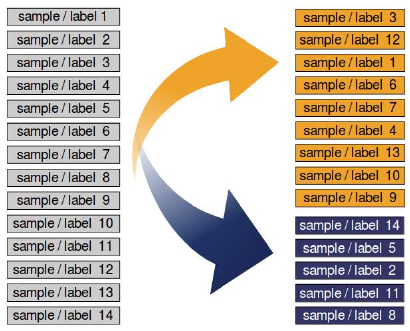
如果数据集按标签排序,我们需要在分割之前打乱它。
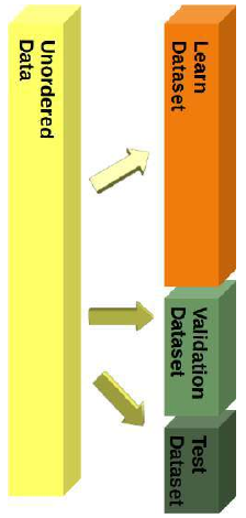
我们将数据集分成了学习(也称为训练)数据集和测试数据集。最佳实践是将其分为学习、测试和评估数据集。
我们将逐步训练我们的模型(分类器),并且每次都需要测试结果。如果我们只有一个测试数据集,测试结果可能会影响模型。因此,我们将使用一个评估数据集来完成整个学习阶段。当我们的分类器完成后,我们再用它从未“见过”的测试数据集来检查它!
然而,在本教程中,我们只会使用学习数据集和测试数据集的分割方式。
分割示例:Iris 数据集
我们将使用 Iris 数据集来演示前面讨论的主题。
Iris 数据集的 150 个数据是排序的,即前 50 个数据对应于第一个花卉类别(0 = Setosa),接下来的 50 个数据对应于第二个花卉类别(1 = Versicolor),其余数据对应于最后一个类别(2 = Virginica)。
如果我们将数据按 2/3(学习集)和 1/3(测试集)的比例分割,那么学习集将包含前两个花卉类别的所有花朵,而测试集将包含第三个花卉类别的所有花朵。这样分类器只能学习两个类别,而第三个类别将完全未知。因此,我们迫切需要将数据混合。
假设所有样本都是相互独立的,我们希望在按照上述方式分割数据集之前,随机打乱数据集。
手动分割数据
下面我们将手动分割数据:
import numpy as np
from sklearn.datasets import load_iris

iris = load_iris()
查看 iris.target 的标签可以发现数据是排序的:
iris.target
Output:array([0, 0, 0, ..., 2, 2, 2])
我们首先要做的就是重新排列数据,使其不再排序。为此,我们将使用 Numpy 的 random 子模块中的 permutation 函数:
indices = np.random.permutation(len(iris.data))
indices
Output:array([ 98, 56, 37, ..., 119, 26, 59])
现在,我们将使用这些随机排列的索引来分割数据:
n_test_samples = 12
learnset_data = iris.data[indices[:-n_test_samples]]
learnset_labels = iris.target[indices[:-n_test_samples]]
testset_data = iris.data[indices[-n_test_samples:]]
testset_labels = iris.target[indices[-n_test_samples:]]

print(learnset_data[:4], learnset_labels[:4])
print(testset_data[:4], testset_labels[:4])
[[5.1 2.5 3.  1.1]
 [6.3 3.3 4.7 1.6]
 [4.9 3.6 1.4 0.1]
 [5.  2.  3.5 1. ]] [1 1 0 1]
[[7.9 3.8 6.4 2. ]
 [5.9 3.  5.1 1.8]
 [6.  2.2 5.  1.5]
 [5.  3.4 1.6 0.4]] [2 2 2 0]
使用 Scikit-learn 进行分割
尽管手动将数据分成学习(训练)集和评估(测试)集并不困难,但我们无需像上面那样手动进行分割。由于这在机器学习中经常需要,scikit-learn 提供了一个预定义的函数来将数据分成训练集和测试集。
我们将在下面演示这一点。我们将使用 80% 的数据作为训练数据,20% 作为测试数据。我们也可以使用 70% 和 30%,因为没有硬性规定。最重要的是,您要根据模型在训练期间未见过的数据来公平地评估您的系统!此外,两个数据集都必须有足够的数据。
from sklearn.datasets import load_iris
from sklearn.model_selection import train_test_split

iris = load_iris()
data, labels = iris.data, iris.target

res = train_test_split(data, labels,
                       train_size=0.8,
                       test_size=0.2,
                       random_state=42)

train_data, test_data, train_labels, test_labels = res

n = 7
print(f"The first {n} data sets:")
print(test_data[:7])
print(f"The corresponding {n} labels:")
print(test_labels[:7])
The first 7 data sets:
[[6.1 2.8 4.7 1.2]
 [5.7 3.8 1.7 0.3]
 [7.7 2.6 6.9 2.3]
 [6.  2.9 4.5 1.5]
 [6.8 2.8 4.8 1.4]
 [5.4 3.4 1.5 0.4]
 [5.6 2.9 3.6 1.3]]
The corresponding 7 labels:
[1 0 2 1 1 0 1]
分层随机抽样
特别是对于相对少量的数据,最好分层进行分割。分层意味着我们保持测试集和训练集中原始数据集的类别比例。我们使用以下代码计算上次分割的类别比例(百分比)。为了计算每个类别出现的次数,我们使用 numpy 函数 bincount。它会计算作为参数传入的非负整数数组中每个值出现的次数。
import numpy as np

print('All:', np.bincount(labels) / float(len(labels)) * 100.0)
print('Training:', np.bincount(train_labels) / float(len(train_labels)) * 100.0)
print('Test:', np.bincount(test_labels) / float(len(test_labels)) * 100.0)
All: [33.33333333 33.33333333 33.33333333]
Training: [33.33333333 34.16666667 32.5       ]
Test: [33.33333333 30.         36.66666667]
为了分层分割,我们可以将标签数组作为附加参数传递给 train_test_split 函数:
from sklearn.datasets import load_iris
from sklearn.model_selection import train_test_split

iris = load_iris()
data, labels = iris.data, iris.target

res = train_test_split(data, labels,
                       train_size=0.8,
                       test_size=0.2,
                       random_state=42,
                       stratify=labels) # 添加 stratify 参数

train_data, test_data, train_labels, test_labels = res

print('All:', np.bincount(labels) / float(len(labels)) * 100.0)
print('Training:', np.bincount(train_labels) / float(len(train_labels)) * 100.0)
print('Test:', np.bincount(test_labels) / float(len(test_labels)) * 100.0)
All: [33.33333333 33.33333333 33.33333333]
Training: [33.33333333 33.33333333 33.33333333]
Test: [33.33333333 33.33333333 33.33333333]
这是一个用来测试分层随机抽样的“愚蠢”例子,因为 Iris 数据集本身就具有相同的比例,即每个类别都有 50 个元素。
我们现在将使用 data 目录中的 strange_flowers.txt 文件。这个数据集是在“使用 Python 生成数据集”一章中创建的。这个数据集中的类别具有不同数量的样本。首先我们加载数据:
content = np.loadtxt("data/strange_flowers.txt", delimiter=" ")
data = content[:, :-1]  # 裁剪掉目标列
labels = content[:, -1]

labels.dtype # 查看标签数据类型
labels.shape # 查看标签形状
Output:(795,)
然后,我们对这个数据应用分层分割:
res = train_test_split(data, labels,
                       train_size=0.8,
                       test_size=0.2,
                       random_state=42,
                       stratify=labels)

train_data, test_data, train_labels, test_labels = res

# np.bincount 期望非负整数:
print('All:', np.bincount(labels.astype(int)) / float(len(labels)) * 100.0)
print('Training:', np.bincount(train_labels.astype(int)) / float(len(train_labels)) * 100.0)
print('Test:', np.bincount(test_labels.astype(int)) / float(len(test_labels)) * 100.0)
All: [ 0.          6.66666667 93.33333333]
Training: [ 0.          6.66666667 93.33333333]
Test: [ 0.          6.66666667 93.33333333]
LEARN, TEST AND EVALUATION DATA
You have your data ready and you are eager to start training the
classifier? But be careful: When your classifier will be finished,
you will need some test data to evaluate your classifier. If you
evaluate your classifier with the data used for learning, you may
see surprisingly good results. What we actually want to test is
the performance of classifying on unknown data.
For this purpose, we need to split our data into two parts:
1.2.A training set with which the learning algorithm
adapts or learns the model
A test set to evaluate the generalization
performance of the model
When you consider how machine learning normally works, the idea of a split between learning and test data
makes sense. Really existing systems train on existing data and if other new data (from customers, sensors or
other sources) comes in, the trained classifier has to predict or classify this new data. We can simulate this
during training with a training and test data set - the test data is a simulation of "future data" that will go into
the system during production.
In this chapter of our Python Machine Learning Tutorial, we will learn how to do the splitting with plain
Python.
We will see also that doing it manually is not necessary, because the train_test_split function from
the model_selection module can do it for us.
If the dataset is sorted by label, we will have to shuffle it before splitting.
65
We separated the dataset into a learn (a.k.a. training) dataset and a test dataset. Best practice is to split it into a
learn, test and an evaluation dataset.
We will train our model (classifier) step by step and each time the result needs to be tested. If we just have a
test dataset. The results of the testing might get into the model. So we will use an evaluation dataset for the
complete learning phase. When our classifier is finished, we will check it with the test dataset, which it has not
"seen" before!
Yet, during our tutorial, we will only use splitings into learn and test datasets.
SPLITTING EXAMPLE: IRIS DATA SET
We will demonstrate the previously discussed topics with the Iris Dataset.
The 150 data sets of the Iris data set are sorted, i.e. the first 50 data correspond to the first flower class (0 =
Setosa), the next 50 to the second flower class (1 = Versicolor) and the remaining data correspond to the last
class (2 = Virginica).
If we were to split our data in the ratio 2/3 (learning set) and 1/3 (test set), the learning set would contain all
the flowers of the first two classes and the test set all the flowers of the third flower class. The classifier could
only learn two classes and the third class would be completely unknown. So we urgently need to mix the data.
Assuming all samples are independent of each other, we want to shuffle the data set randomly before we split
the data set as shown above.
66
In the following we split the data manually:
import numpy as np
from sklearn.datasets import load_iris
iris = load_iris()
Looking at the labels of iris.target shows us that the data is sorted.
iris.target
Output:array([0, 0, 0, 0, 0, 0, 0, 0, 0, 0, 0, 0, 0, 0, 0, 0, 0, 0,
0, 0, 0, 0,
0, 0, 0, 0, 0, 0, 0, 0, 0, 0, 0, 0, 0, 0, 0, 0, 0, 0,
0, 0, 0, 0,
0, 0, 0, 0, 0, 0, 1, 1, 1, 1, 1, 1, 1, 1, 1, 1, 1, 1,
1, 1, 1, 1,
1, 1, 1, 1, 1, 1, 1, 1, 1, 1, 1, 1, 1, 1, 1, 1, 1, 1,
1, 1, 1, 1,
1, 1, 1, 1, 1, 1, 1, 1, 1, 1, 1, 1, 2, 2, 2, 2, 2, 2,
2, 2, 2, 2,
2, 2, 2, 2, 2, 2, 2, 2, 2, 2, 2, 2, 2, 2, 2, 2, 2, 2,
2, 2, 2, 2,
2, 2, 2, 2, 2, 2, 2, 2, 2, 2, 2, 2, 2, 2, 2, 2, 2, 2])
The first thing we have to do is rearrange the data so that it is not sorted anymore. For this purpose, we will
use the permutation function of the random submodul of Numpy:
indices = np.random.permutation(len(iris.data))
indices
67
Output:array([ 98,
56,
37,
60,
94, 142, 117, 121,
10,
15,
8
9,
85,
66,
29, 44, 102, 24, 140, 58, 25, 19, 100, 83, 12
6, 28, 118,
50, 127, 72, 99, 74,
0, 128, 11, 45, 143, 5
4, 79, 34,
32, 95, 92, 46, 146,
3,
9, 73, 101, 23, 7
7, 39, 87,
111, 129, 148, 67, 75, 147, 48, 76, 43, 30, 14
4, 27, 104,
35, 93, 125,
2, 69, 63, 40, 141,
7, 133, 1
8,
4, 12,
109, 33, 88, 71, 22, 110, 42,
8, 134,
5, 9
7, 114, 135,
108, 91, 14,
6, 137, 124, 130, 145, 55, 17, 8
0, 36, 61,
49, 62, 90, 84, 64, 139, 107, 112,
1, 70, 12
3, 38, 132,
31, 16, 13, 21, 113, 120, 41, 106, 65, 20, 11
6, 86, 68,
96, 78, 53, 47, 105, 136, 51, 57, 131, 149, 11
9, 26, 59,
138, 122, 81, 103, 52, 115, 82])
n_test_samples = 12
learnset_data = iris.data[indices[:-n_test_samples]]
learnset_labels = iris.target[indices[:-n_test_samples]]
testset_data = iris.data[indices[-n_test_samples:]]
testset_labels = iris.target[indices[-n_test_samples:]]
print(learnset_data[:4], learnset_labels[:4])
print(testset_data[:4], testset_labels[:4])
[[5.1 2.5 3. 1.1]
[6.3 3.3 4.7 1.6]
[4.9 3.6 1.4 0.1]
[5. 2. 3.5 1. ]] [1 1 0 1]
[[7.9 3.8 6.4 2. ]
[5.9 3. 5.1 1.8]
[6. 2.2 5. 1.5]
[5. 3.4 1.6 0.4]] [2 2 2 0]
SPLITS WITH SKLEARN
Even though it was not difficult to split the data manually into a learn (train) and an evaluation (test) set, we
don't have to do the splitting manually as shown above. Since this is often required in machine learning, scikit-
learn has a predefined function for dividing data into training and test sets.
68
We will demonstrate this below. We will use 80% of the data as training and 20% as test data. We could just as
well have taken 70% and 30%, because there are no hard and fast rules. The most important thing is that you
rate your system fairly based on data it did not see during exercise! In addition, there must be enough data in
both data sets.
from sklearn.datasets import load_iris
from sklearn.model_selection import train_test_split
iris = load_iris()
data, labels = iris.data, iris.target
res = train_test_split(data, labels,
train_size=0.8,
test_size=0.2,
random_state=42)
train_data, test_data, train_labels, test_labels = res
n = 7
print(f"The first {n} data sets:")
print(test_data[:7])
print(f"The corresponding {n} labels:")
print(test_labels[:7])
The first 7 data sets:
[[6.1 2.8 4.7 1.2]
[5.7 3.8 1.7 0.3]
[7.7 2.6 6.9 2.3]
[6. 2.9 4.5 1.5]
[6.8 2.8 4.8 1.4]
[5.4 3.4 1.5 0.4]
[5.6 2.9 3.6 1.3]]
The corresponding 7 labels:
[1 0 2 1 1 0 1]
STRATIFIED RANDOM SAMPLE
Especially with relatively small amounts of data, it is better to stratify the division. Stratification means that
we keep the original class proportion of the data set in the test and training sets. We calculate the class
proportions of the previous split in percent using the following code. To calculate the number of occurrences
of each class, we use the numpy function 'bincount'. It counts the number of occurrences of each value in the
array of non-negative integers passed as an argument.
import numpy as np
print('All:', np.bincount(labels) / float(len(labels)) * 100.0)
print('Training:', np.bincount(train_labels) / float(len(train_lab
els)) * 100.0)
69
print('Test:', np.bincount(test_labels) / float(len(test_labels))
* 100.0)
All: [33.33333333 33.33333333 33.33333333]
Training: [33.33333333 34.16666667 32.5
Test: [33.33333333 30.
36.66666667]
]
To stratify the division, we can pass the label array as an additional argument to the train_test_split function:
from sklearn.datasets import load_iris
from sklearn.model_selection import train_test_split
iris = load_iris()
data, labels = iris.data, iris.target
res = train_test_split(data, labels,
train_size=0.8,
test_size=0.2,
random_state=42,
stratify=labels)
train_data, test_data, train_labels, test_labels = res
print('All:', np.bincount(labels) / float(len(labels)) * 100.0)
print('Training:', np.bincount(train_labels) / float(len(train_lab
els)) * 100.0)
print('Test:', np.bincount(test_labels) / float(len(test_labels))
* 100.0)
All: [33.33333333 33.33333333 33.33333333]
Training: [33.33333333 33.33333333 33.33333333]
Test: [33.33333333 33.33333333 33.33333333]
This was a stupid example to test the stratified random sample, because the Iris data set has the same
proportions, i.e. each class 50 elements.
We will work now with the file strange_flowers.txt of the directory data . This data set is created
in the chapter Generate Datasets in Python The classes in this dataset have different numbers of items. First
we load the data:
content = np.loadtxt("data/strange_flowers.txt", delimiter=" ")
data = content[:, :-1]
# cut of the target column
labels = content[:, -1]
labels.dtype
labels.shape
Output795,)
70
res = train_test_split(data, labels,
train_size=0.8,
test_size=0.2,
random_state=42,
stratify=labels)
train_data, test_data, train_labels, test_labels = res
# np.bincount expects non negative integers:
print('All:', np.bincount(labels.astype(int)) / float(len(label
s)) * 100.0)
print('Training:', np.bincount(train_labels.astype(int)) / float(l
en(train_labels)) * 100.0)
print('Test:', np.bincount(test_labels.astype(int)) / float(len(te
st_labels)) * 100.0)
All: [ 0.
Training: [ 0.
478 ]
Test: [ 0.
]