机器学习Python教程
 使用 Scikit-learn / SKLearn 构建神经网络
简介
在本教程的先前章节中,我们手动创建了神经网络。这是为了深入理解神经网络的实现方式。这种理解对于使用 Python sklearn 模块提供的分类器非常有用。在本章中,我们将使用 sklearn.neural_network 中包含的多层感知器分类器 (MLPClassifier)。
我们将再次使用 Iris 数据集来介绍这个分类器,这个数据集在我们之前的 Python 机器学习教程中已经多次使用。
MLPClassifier 分类器
我们将继续使用多层感知器 (MLP) 的例子。多层感知器 (MLP) 是一种前馈人工神经网络模型,它将输入数据集映射到一组适当的输出。MLP 由多个层组成,每层都与下一层完全连接。各层中的节点都是使用非线性激活函数的神经元,输入层的节点除外。在输入层和输出层之间可以有一个或多个非线性隐藏层。
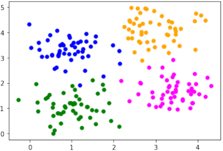
多标签示例
import matplotlib.pyplot as plt
from sklearn.datasets import make_blobs

n_samples = 200
blob_centers = ([1, 1], [3, 4], [1, 3.3], [3.5, 1.8])
data, labels = make_blobs(n_samples=n_samples,
centers=blob_centers,
cluster_std=0.5,
random_state=0)

colours = ('green', 'orange', "blue", "magenta")
fig, ax = plt.subplots()
for n_class in range(len(blob_centers)):
    ax.scatter(data[labels==n_class][:, 0],
    data[labels==n_class][:, 1],
    c=colours[n_class],
    s=30,
    label=str(n_class))
plt.show() # 添加这行来显示图表


from sklearn.model_selection import train_test_split
datasets = train_test_split(data,
labels,
test_size=0.2)
train_data, test_data, train_labels, test_labels = datasets
from sklearn.model_selection import train_test_split
datasets = train_test_split(data,
labels,
test_size=0.2)
train_data, test_data, train_labels, test_labels = datasets
现在我们将创建一个 MLPClassifier。
关于所用参数的一些说明:
-
hidden_layer_sizes: 元组,长度 = n_layers - 2,默认值为 (100,)。
第 i 个元素表示第 i 个隐藏层中的神经元数量。
例如,(6,) 表示一个包含 6 个神经元的隐藏层。
-
solver:
权重优化可以通过 solver 参数来控制。有三种求解器模式可用:
-
'lbfgs'是一种准牛顿方法族的优化器。 -
'sgd'指随机梯度下降。 -
'adam' 指 Kingma, Diederik 和 Jimmy Ba 提出的基于随机梯度的优化器。
在不深入了解求解器细节的情况下,您应该了解以下内容:'adam' 在相对大型的数据集(即数千个训练样本或更多)上表现非常好——无论是训练时间还是验证分数。然而,对于小型数据集,'lbfgs' 可以更快地收敛并表现更好。
-
-
'alpha':
此参数可用于控制可能的“过拟合”和“欠拟合”。我们将在本章后面详细介绍它。
from sklearn.neural_network import MLPClassifier
clf = MLPClassifier(solver='lbfgs',
alpha=1e-5,
hidden_layer_sizes=(6,),
random_state=1)
clf.fit(train_data, train_labels)
print(clf)
Output:
MLPClassifier(alpha=1e-05, hidden_layer_sizes=(6,), random_state=1,
solver='lbfgs')
print(clf.score(train_data, train_labels))
Output:
1.0
from sklearn.metrics import accuracy_score
predictions_train = clf.predict(train_data)
predictions_test = clf.predict(test_data)
train_score = accuracy_score(predictions_train, train_labels)
print("score on train data: ", train_score)
test_score = accuracy_score(predictions_test, test_labels)
print("score on test data: ", test_score) # 修正输出为 test data
Output:
score on train data:  1.0
score on test data:  0.95
print(predictions_train[:20])
Output:
array([2, 0, 1, 0, 2, 1, 3, 0, 3, 0, 2, 2, 1, 1, 0, 0, 1, 2, 2, 3])
多层感知器
from sklearn.neural_network import MLPClassifier
X = [[0., 0.], [0., 1.], [1., 0.], [1., 1.]]
y = [0, 0, 0, 1]
clf = MLPClassifier(solver='lbfgs', alpha=1e-5,
hidden_layer_sizes=(5, 2), random_state=1)
print(clf.fit(X, y))
Output:
MLPClassifier(alpha=1e-05, hidden_layer_sizes=(5, 2), random_state=1,
solver='lbfgs')
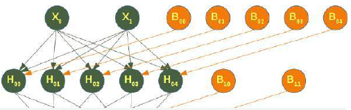
下图描绘了我们为分类器 clf 训练的神经网络。我们有两个输入节点 \(X_0\) 和 \(X_1\),称为输入层,以及一个输出神经元 'Out'。我们有两个隐藏层,第一个包含神经元 \(H_00\) ... \(H_04\),第二个隐藏层包含 \(H_10\) 和 \(H_11\)。隐藏层的每个神经元和输出神经元都具有相应的偏差 (Bias),即 \(B_00\) 是神经元 \(H_00\) 的相应偏差,\(B_01\) 是神经元 \(H_01\) 的相应偏差,依此类推。
隐藏层的每个神经元都接收来自前一层每个神经元的输出,并通过加权线性求和:
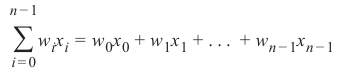
将其转换为输出值,其中 n 是层中的神经元数量,w_i 对应于权重向量的第 i 个分量。输出层接收来自最后一个隐藏层的值。它也执行线性求和,但会将非线性激活函数:
(例如双曲正切函数)应用于求和结果。
属性 coefs_ 包含每层的权重矩阵列表。索引 i 处的权重矩阵包含层 i 和层 i + 1 之间的权重。
print("输入层和第一个隐藏层之间的权重:")
print(clf.coefs_[0])
print("\n第一个隐藏层和第二个隐藏层之间的权重:")
print(clf.coefs_[1])
神经元 \(H_00\) 的求和公式定义为:
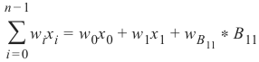
可以写成:
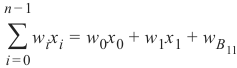
因为\(B_11=1\)。
我们可以像这样从 clf.coefs_ 获取 \(w_0\) 和 \(w_1\) 的值:
\(w_0=\text{clf.coefs_[0][0][0]}\) 和 \(w_1=\text{clf.coefs_[0][1][0]}\)
print("w0 = ", clf.coefs_[0][0][0])
print("w1 = ", clf.coefs_[0][1][0])
可以通过以下方式访问神经元 \(H_00\) 的权重向量:
print(clf.coefs_[0][:,0])
我们可以将上述内容推广到以下方式访问神经元 \(H_ij\):
for i in range(len(clf.coefs_)):
    number_neurons_in_layer = clf.coefs_[i].shape[1]
    for j in range(number_neurons_in_layer):
        weights = clf.coefs_[i][:,j]
        print(i, j, weights, end=", ")
    print()
    print()
intercepts_ 是偏差向量的列表,其中索引 i 处的向量表示添加到层 i+1 的偏差值。
print("第一个隐藏层的偏差值:")
print(clf.intercepts_[0])
print("\n第二个隐藏层的偏差值:")
print(clf.intercepts_[1])
我们训练分类器的主要原因是预测新样本的结果。我们可以使用 predict 方法来完成此操作。该方法为样本返回一个预测类别,在我们的例子中是“0”或“1”:
result = clf.predict([[0, 0], [0, 1],
[1, 0], [0, 1],
[1, 1], [2., 2.],
[1.3, 1.3], [2, 4.8]])
print(result) # 添加这行来显示结果
除了查看类别结果,我们还可以使用 predict_proba 方法来获取概率估计。
prob_results = clf.predict_proba([[0, 0], [0, 1],
[1, 0], [0, 1],
[1, 1], [2., 2.],
[1.3, 1.3], [2, 4.8]])
print(prob_results)
prob_results[i][0] 给出了类别 0 的概率(即“0”),prob_results[i][1] 给出了类别 1 的概率(即“1”)。i 对应于第 i 个样本。
完整的 Iris 数据集示例
from sklearn.datasets import load_iris
iris = load_iris()
# 将数据拆分为训练集和测试集
from sklearn.model_selection import train_test_split
datasets = train_test_split(iris.data, iris.target,
test_size=0.2)
train_data, test_data, train_labels, test_labels = datasets
# 数据缩放
from sklearn.preprocessing import StandardScaler
scaler = StandardScaler()
# 我们在训练数据上拟合
scaler.fit(train_data)
# 缩放训练数据
train_data = scaler.transform(train_data)
test_data = scaler.transform(test_data)
print(train_data[:3])
Output:
[[ 1.91343191 -0.6013337   1.31398787  0.89583493]
[-0.93504278  1.48689909 -1.31208492 -1.08512683]
[ 0.4272712  -0.36930784  0.28639417  0.10345022]]
训练模型
from sklearn.neural_network import MLPClassifier
# 从模型创建分类器:
mlp = MLPClassifier(hidden_layer_sizes=(10, 5), max_iter=1000)
# 让我们将训练数据拟合到我们的模型中
mlp.fit(train_data, train_labels)
print(mlp)
Output:
MLPClassifier(hidden_layer_sizes=(10, 5), max_iter=1000)
from sklearn.metrics import accuracy_score
predictions_train = mlp.predict(train_data)
print(accuracy_score(predictions_train, train_labels))
predictions_test = mlp.predict(test_data)
print(accuracy_score(predictions_test, test_labels))
Output:
0.975
0.9666666666666667
from sklearn.metrics import confusion_matrix
print(confusion_matrix(predictions_train, train_labels))
Output:
array([[42,  0,  0],
       [ 0, 37,  1],
       [ 0,  2, 38]])
print(confusion_matrix(predictions_test, test_labels))
Output:
array([[ 8,  0,  0],
       [ 0, 10,  0],
       [ 0,  1, 11]])
from sklearn.metrics import classification_report
print(classification_report(predictions_test, test_labels))
Output:
              precision    recall  f1-score   support

           0       1.00      1.00      1.00         8
           1       0.91      1.00      0.95        10
           2       1.00      0.92      0.96        12

    accuracy                           0.97        30
   macro avg       0.97      0.97      0.97        30
weighted avg       0.97      0.97      0.97        30
MNIST 数据集
我们已经在教程的“使用 MNIST 进行测试”一章中使用了 MNIST 数据集。您还可以在该章中找到关于此数据集的一些解释。
我们想将 MLPClassifier 应用于 MNIST 数据。我们可以使用 pickle 加载数据:
import pickle
with open("data/mnist/pickled_mnist.pkl", "br") as fh:
    data = pickle.load(fh)
train_imgs = data[0]
test_imgs = data[1]
train_labels = data[2]
test_labels = data[3]
train_labels_one_hot = data[4]
test_labels_one_hot = data[5]

image_size = 28 # 宽度和长度
no_of_different_labels = 10 # 即 0, 1, 2, 3, ..., 9
image_pixels = image_size * image_size

mlp = MLPClassifier(hidden_layer_sizes=(100, ),
max_iter=480, alpha=1e-4,
solver='sgd', verbose=10,
tol=1e-4, random_state=1,
learning_rate_init=.1)
train_labels = train_labels.reshape(train_labels.shape[0],)
print(train_imgs.shape, train_labels.shape)
mlp.fit(train_imgs, train_labels)
print("Training set score: %f" % mlp.score(train_imgs, train_labels))
print("Test set score: %f" % mlp.score(test_imgs, test_labels))
Output:
(60000, 784) (60000,)
Iteration 1, loss = 0.29753549
Iteration 2, loss = 0.12369769
Iteration 3, loss = 0.08872688
Iteration 4, loss = 0.07084598
Iteration 5, loss = 0.05874947
Iteration 6, loss = 0.04876359
Iteration 7, loss = 0.04203350
Iteration 8, loss = 0.03525624
Iteration 9, loss = 0.02995642
Iteration 10, loss = 0.02526208
Iteration 11, loss = 0.02195436
Iteration 12, loss = 0.01825246
Iteration 13, loss = 0.01543440
Iteration 14, loss = 0.01320164
Iteration 15, loss = 0.01057486
Iteration 16, loss = 0.00984482
Iteration 17, loss = 0.00776886
Iteration 18, loss = 0.00655891
Iteration 19, loss = 0.00539189
Iteration 20, loss = 0.00460981
Iteration 21, loss = 0.00396910
Iteration 22, loss = 0.00350800
Iteration 23, loss = 0.00328115
Iteration 24, loss = 0.00294118
Iteration 25, loss = 0.00265852
Iteration 26, loss = 0.00241809
Iteration 27, loss = 0.00234944
Iteration 28, loss = 0.00215147
Iteration 29, loss = 0.00201855
Iteration 30, loss = 0.00187808
Iteration 31, loss = 0.00183098
Iteration 32, loss = 0.00172363
Iteration 33, loss = 0.00169482
Iteration 34, loss = 0.00159811
Iteration 35, loss = 0.00152427
Iteration 36, loss = 0.00148731
Iteration 37, loss = 0.00144202
Iteration 38, loss = 0.00138101
Iteration 39, loss = 0.00133767
Iteration 40, loss = 0.00130437
Iteration 41, loss = 0.00126314
Iteration 42, loss = 0.00122969
Iteration 43, loss = 0.00119848
Training loss did not improve more than tol=0.000100 for 10 consecutive epochs. Stopping.
Training set score: 1.000000
Test set score: 0.977900
sklearn.neural_network._multilayer_perceptron 模块中 fit 方法的帮助信息:
fit(X, y) 方法属于 sklearn.neural_network._multilayer_perceptron.MLPClassifier 实例。
将模型拟合到数据矩阵 X 和目标 y。
参数
X : ndarray 或稀疏矩阵,形状为 (n_samples, n_features)
输入数据。
y : ndarray,形状为 (n_samples,) 或 (n_samples, n_outputs)
目标值(分类中的类别标签,回归中的实数)。
返回
self : 返回一个训练好的 MLP 模型。
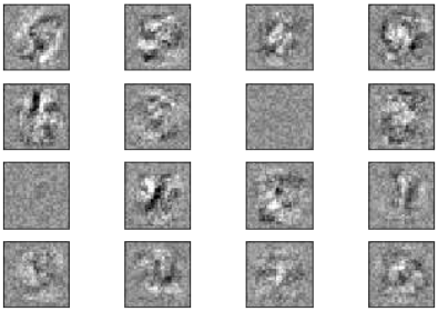
import matplotlib.pyplot as plt # 确保导入
fig, axes = plt.subplots(4, 4)
# 使用全局最小值 / 最大值以确保所有权重都在相同的比例尺上显示
vmin, vmax = mlp.coefs_[0].min(), mlp.coefs_[0].max()
for coef, ax in zip(mlp.coefs_[0].T, axes.ravel()):
    ax.matshow(coef.reshape(28, 28), cmap=plt.cm.gray, vmin=.5 * vmin,
    vmax=.5 * vmax)
    ax.set_xticks(())
    ax.set_yticks(())
plt.show()
参数 Alpha
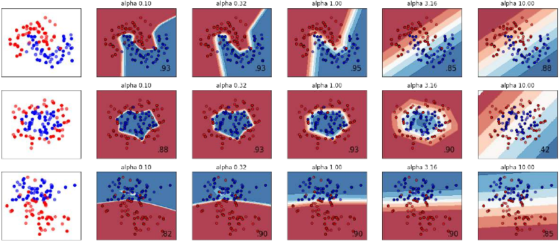
在合成数据集上比较正则化参数 ‘alpha’ 的不同值。该图显示了不同的 alpha 值会产生不同的决策函数。
Alpha 是正则化项(又称惩罚项)的参数,通过限制权重的大小来对抗过拟合。增加 alpha 可以通过鼓励更小的权重来修复高方差(过拟合的迹象),从而使决策边界图的曲率更小。类似地,减小 alpha 可以通过鼓励更大的权重来修复高偏差(欠拟合的迹象),从而可能导致更复杂的决策边界。
作者: Issam H. Laradji
许可证: BSD 3 clause
代码来源: https://scikit-learn.org/stable/auto_examples/neural_networks/plot_mlp_alpha.html
import numpy as np
from matplotlib import pyplot as plt
from matplotlib.colors import ListedColormap
from sklearn.model_selection import train_test_split
from sklearn.preprocessing import StandardScaler
from sklearn.datasets import make_moons, make_circles, make_classification
from sklearn.neural_network import MLPClassifier
from sklearn.pipeline import make_pipeline

h = .02  # 网格中的步长
alphas = np.logspace(-1, 1, 5) # 生成在 0.1 到 10 之间对数等距的 5 个值

classifiers = []
names = []
for alpha in alphas:
    classifiers.append(make_pipeline(
    StandardScaler(),
    MLPClassifier(
    solver='lbfgs', alpha=alpha, random_state=1, max_iter=2000,
    early_stopping=True, hidden_layer_sizes=[100, 100],
    )
    ))
    names.append(f"alpha {alpha:<span class="hljs-number">.2</span>f}")

X, y = make_classification(n_features=2, n_redundant=0, n_informative=2,
random_state=0, n_clusters_per_class=1)
rng = np.random.RandomState(2)
X += 2 * rng.uniform(size=X.shape)
linearly_separable = (X, y)
datasets = [make_moons(noise=0.3, random_state=0),
make_circles(noise=0.2, factor=0.5, random_state=1),
linearly_separable]
figure = plt.figure(figsize=(17, 9))
i = 1
# 遍历数据集
for X, y in datasets:
    # 拆分为训练和测试部分
    X_train, X_test, y_train, y_test = train_test_split(X, y, test_size=.4)
    x_min, x_max = X[:, 0].min() - .5, X[:, 0].max() + .5
    y_min, y_max = X[:, 1].min() - .5, X[:, 1].max() + .5
    xx, yy = np.meshgrid(np.arange(x_min, x_max, h),
    np.arange(y_min, y_max, h))
    # 首先只绘制数据集
    cm = plt.cm.RdBu
    cm_bright = ListedColormap(['#FF0000', '#0000FF'])
    ax = plt.subplot(len(datasets), len(classifiers) + 1, i)
    # 绘制训练点
    ax.scatter(X_train[:, 0], X_train[:, 1], c=y_train, cmap=cm_bright)
    # 绘制测试点
    ax.scatter(X_test[:, 0], X_test[:, 1], c=y_test, cmap=cm_bright, alpha=0.6)
    ax.set_xlim(xx.min(), xx.max())
    ax.set_ylim(yy.min(), yy.max())
    ax.set_xticks(())
    ax.set_yticks(())
    i += 1
    # 遍历分类器
    for name, clf in zip(names, classifiers):
        ax = plt.subplot(len(datasets), len(classifiers) + 1, i)
        clf.fit(X_train, y_train)
        score = clf.score(X_test, y_test)
        # 绘制决策边界。为此,我们将为网格中的每个点分配颜色 [x_min, x_max] x [y_min, y_max]。
        if hasattr(clf, "decision_function"):
            Z = clf.decision_function(np.c_[xx.ravel(), yy.ravel()])
        else:
            Z = clf.predict_proba(np.c_[xx.ravel(), yy.ravel()])[:, 1]
        # 将结果放入颜色图中
        Z = Z.reshape(xx.shape)
        ax.contourf(xx, yy, Z, cmap=cm, alpha=.8)
        # 绘制训练点
        ax.scatter(X_train[:, 0], X_train[:, 1], c=y_train, cmap=cm_bright,
        edgecolors='black', s=25)
        # 绘制测试点
        ax.scatter(X_test[:, 0], X_test[:, 1], c=y_test, cmap=cm_bright,
        alpha=0.6, edgecolors='black', s=25)
        ax.set_xlim(xx.min(), xx.max())
        ax.set_ylim(yy.min(), yy.max())
        ax.set_xticks(())
        ax.set_yticks(())
        ax.set_title(name)
        ax.text(xx.max() - .3, yy.min() + .3, ('%.2f' % score).lstrip('0'),
        size=15, horizontalalignment='right')
        i += 1
figure.subplots_adjust(left=.02,right=.98)
plt.show()
练习
练习 1
使用 K 最近邻分类器对 “strange_flowers.txt” 中的数据进行分类。
解决方案
练习 1 解决方案
我们使用 pandas 模块的 read_csv 来读取 strange_flowers.txt 文件:
import pandas as pd
dataset = pd.read_csv("data/strange_flowers.txt",
header=None,
names=["red", "green", "blue", "size", "label"],
sep=" ")
print(dataset)
Output:
      red  green  blue  size  label
0   238.0  104.0   8.0  3.65    1.0
1   235.0  114.0   9.0  4.00    1.0
2   252.0   93.0   9.0  3.71    1.0
3   242.0  116.0   9.0  3.67    1.0
4   251.0  117.0  15.0  3.49    1.0
...   ...    ...   ...   ...    ...
790   0.0  248.0  98.0  3.03    4.0
791   0.0  253.0 106.0  2.85    4.0
792   0.0  250.0  91.0  3.39    4.0
793   0.0  248.0  99.0  3.10    4.0
794   0.0  244.0 109.0  2.96    4.0

[795 rows x 5 columns]
前四列包含数据,最后一列包含标签:
data = dataset.drop('label', axis=1)
labels = dataset.label
from sklearn.model_selection import train_test_split
X_train, X_test, y_train, y_test = train_test_split(data,
labels,
random_state=0,
test_size=0.2)
现在我们必须对数据进行缩放,以减少数据之间的偏差:
from sklearn.preprocessing import StandardScaler
scaler = StandardScaler()
X_train = scaler.fit_transform(X_train) # transform
X_test = scaler.transform(X_test) # transform
from sklearn.neural_network import MLPClassifier
mlp = MLPClassifier(hidden_layer_sizes=(100, ),
max_iter=480,
alpha=1e-4,
solver='sgd',
tol=1e-4,
random_state=1,
learning_rate_init=.1)
mlp.fit(X_train, y_train)
print("Training set score: %f" % mlp.score(X_train, y_train))
print("Test set score: %f" % mlp.score(X_test, y_test))
Output:
Training set score: 0.971698
Test set score: 0.981132
NEURAL NETWORKS WITH SCIKIT /
SKLEARN
INTRODUCTION
In the previous chapters of our tutorial, we
manually created Neural Networks. This
was necessary to get a deep understanding
of how Neural networks can be
implemented. This understanding is very
useful to use the classifiers provided by
the sklearn module of Python. In this
chapter we will use the multilayer
perceptron classifier MLPClassifier
contained in
sklearn.neural_network
We will use again the Iris dataset, which
we had used already multiple times in our
Machine Learning tutorial with Python, to
introduce this classifier.
MLPCLASSIFIER
CLASSIFIER
We will continue with examples using the multilayer perceptron (MLP). The multilayer perceptron (MLP) is a
feedforward artificial neural network model that maps sets of input data onto a set of appropriate outputs. An
MLP consists of multiple layers and each layer is fully connected to the following one. The nodes of the layers
are neurons using nonlinear activation functions, except for the nodes of the input layer. There can be one or
more non-linear hidden layers between the input and the output layer.
MULTILABEL EXAMPLE
import matplotlib.pyplot as plt
from sklearn.datasets import make_blobs
n_samples = 200
blob_centers = ([1, 1], [3, 4], [1, 3.3], [3.5, 1.8])
data, labels = make_blobs(n_samples=n_samples,
centers=blob_centers,
cluster_std=0.5,
random_state=0)
252
colours = ('green', 'orange', "blue", "magenta")
fig, ax = plt.subplots()
for n_class in range(len(blob_centers)):
ax.scatter(data[labels==n_class][:, 0],
data[labels==n_class][:, 1],
c=colours[n_class],
s=30,
label=str(n_class))
from sklearn.model_selection import train_test_split
datasets = train_test_split(data,
labels,
test_size=0.2)
train_data, test_data, train_labels, test_labels = datasets
We will create now a MLPClassifier .
A few notes on the used parameters:
•hidden_layer_sizes: tuple, length = n_layers - 2, default=(100,)
The ith element represents the number of neurons in the ith hidden layer.
(6,) means one hidden layer with 6 neurons
• solver:
The weight optimization can be influenced with the solver parameter. Three solver modes
are available
▪'lbfgs'
is an optimizer in the family of quasi-Newton methods.
253
▪▪'sgd'
refers to stochastic gradient descent.
'adam' refers to a stochastic gradient-based optimizer proposed by Kingma,
Diederik, and Jimmy Ba
Without understanding in the details of the solvers, you should know the following: 'adam'
works pretty well - both training time and validation score - on relatively large datasets, i.e.
thousands of training samples or more. For small datasets, however, 'lbfgs' can converge faster
and perform better.
•'alpha'
This parameter can be used to control possible 'overfitting' and 'underfitting'. We will cover it in
detail further down in this chapter.
from sklearn.neural_network import MLPClassifier
clf = MLPClassifier(solver='lbfgs',
alpha=1e-5,
hidden_layer_sizes=(6,),
random_state=1)
clf.fit(train_data, train_labels)
Output:MLPClassifier(alpha=1e-05, hidden_layer_sizes=(6,), random_st
ate=1,
solver='lbfgs')
clf.score(train_data, train_labels)
Output:1.0
from sklearn.metrics import accuracy_score
predictions_train = clf.predict(train_data)
predictions_test = clf.predict(test_data)
train_score = accuracy_score(predictions_train, train_labels)
print("score on train data: ", train_score)
test_score = accuracy_score(predictions_test, test_labels)
print("score on train data: ", test_score)
score on train data:
1.0
score on train data:
0.95
predictions_train[:20]
Output:array([2, 0, 1, 0, 2, 1, 3, 0, 3, 0, 2, 2, 1, 1, 0, 0, 1, 2,
2, 3])
254
MULTI-LAYER PERCEPTRON
from sklearn.neural_network import MLPClassifier
X = [[0., 0.], [0., 1.], [1., 0.], [1., 1.]]
y = [0, 0, 0, 1]
clf = MLPClassifier(solver='lbfgs', alpha=1e-5,
hidden_layer_sizes=(5, 2), random_state=1)
print(clf.fit(X, y))
MLPClassifier(alpha=1e-05, hidden_layer_sizes=(5, 2), random_stat
e=1,
solver='lbfgs')
The following diagram depicts the neural network, that we have trained for our classifier clf. We have two
input nodes X 0 and X 1, called the input layer, and one output neuron 'Out'. We have two hidden layers the first
one with the neurons H 00 ... H 04 and the second hidden layer consisting of H10 and H 11. Each neuron of the
hidden layers and the output neuron possesses a corresponding Bias, i.e. B00 is the corresponding Bias to the
neuron H 00, B 01 is the corresponding Bias to the neuron H01 and so on.
Each neuron of the hidden layers receives the output from every neuron of the previous layers and transforms
these values with a weighted linear summation
n −1
∑ w ix i = w 0x 0 + w1x 1 + . . . + w n − 1x n − 1
i =0
into an output value, where n is the number of neurons of the layer and wi corresponds to the ith component of
the weight vector. The output layer receives the values from the last hidden layer. It also performs a linear
summation, but a non-linear activation function
g( ⋅ ) : R → R
like the hyperbolic tan function will be applied to the summation result.
255
The attribute coefs_ contains a list of
weight matrices for every layer. The
weight matrix at index i holds the weights
between the layer i and layer i + 1.
In [ ]:
print("weights between in
put and first hidden laye
r:")
print(clf.coefs_[0])
print("\nweights between
first hidden and second h
idden layer:")
print(clf.coefs_[1])
The summation formula of the neuron H00 is defined by:
n −1
∑ w ix i = w 0x 0 + w1x 1 + w B11 ∗ B11
i =0
which can be written as
n −1
∑ w ix i = w0x 0 + w 1x 1 + w B11
i =0
because B = 1.
11We can get the values for w 0 and w 1 from clf.coefs_ like this:
w 0 = clf.coefs_[0][0][0] and w1 = clf.coefs_[0][1][0]
In [ ]:
print("w0 = ", clf.coefs_[0][0][0])
print("w1 = ", clf.coefs_[0][1][0])
The weight vector of H can be accessed with
00In [ ]:
clf.coefs_[0][:,0]
256
We can generalize the above to access a neuron H in the following way:
ijIn [ ]:
for i in range(len(clf.coefs_)):
number_neurons_in_layer = clf.coefs_[i].shape[1]
for j in range(number_neurons_in_layer):
weights = clf.coefs_[i][:,j]
print(i, j, weights, end=", ")
print()
print()
intercepts_ is a list of bias vectors, where the vector at index i represents the bias values added to layer i+1.
In [ ]:
print("Bias values for first hidden layer:")
print(clf.intercepts_[0])
print("\nBias values for second hidden layer:")
print(clf.intercepts_[1])
The main reason, why we train a classifier is to predict results for new samples. We can do this with the
predict method. The method returns a predicted class for a sample, in our case a "0" or a "1" :
In [ ]:
result = clf.predict([[0, 0], [0, 1],
[1, 0], [0, 1],
[1, 1], [2., 2.],
[1.3, 1.3], [2, 4.8]])
Instead of just looking at the class results, we can also use the predict_proba method to get the probability
estimates.
In [ ]:
prob_results = clf.predict_proba([[0, 0], [0, 1],
[1, 0], [0, 1],
[1, 1], [2., 2.],
[1.3, 1.3], [2, 4.8]])
print(prob_results)
prob_results[i][0] gives us the probability for the class0, i.e. a "0" and results[i][1] the probabilty for a "1". i
corresponds to the ith sample.
COMPLETE IRIS DATASET EXAMPLE
257
from sklearn.datasets import load_iris
iris = load_iris()
# splitting into train and test datasets
from sklearn.model_selection import train_test_split
datasets = train_test_split(iris.data, iris.target,
test_size=0.2)
train_data, test_data, train_labels, test_labels = datasets
# scaling the data
from sklearn.preprocessing import StandardScaler
scaler = StandardScaler()
# we fit the train data
scaler.fit(train_data)
# scaling the train data
train_data = scaler.transform(train_data)
test_data = scaler.transform(test_data)
print(train_data[:3])
[[ 1.91343191 -0.6013337
1.31398787 0.89583493]
[-0.93504278 1.48689909 -1.31208492 -1.08512683]
[ 0.4272712 -0.36930784 0.28639417 0.10345022]]
# Training the Model
from sklearn.neural_network import MLPClassifier
# creating an classifier from the model:
mlp = MLPClassifier(hidden_layer_sizes=(10, 5), max_iter=1000)
# let's fit the training data to our model
mlp.fit(train_data, train_labels)
Output:MLPClassifier(hidden_layer_sizes=(10, 5), max_iter=1000)
from sklearn.metrics import accuracy_score
predictions_train = mlp.predict(train_data)
print(accuracy_score(predictions_train, train_labels))
predictions_test = mlp.predict(test_data)
print(accuracy_score(predictions_test, test_labels))
258
0.975
0.9666666666666667
from sklearn.metrics import confusion_matrix
confusion_matrix(predictions_train, train_labels)
Output:array([[42,
0, 0],
[ 0, 37, 1],
[ 0, 2, 38]])
confusion_matrix(predictions_test, test_labels)
Output:array([[ 8,
0, 0],
[ 0, 10, 0],
[ 0, 1, 11]])
from sklearn.metrics import classification_report
print(classification_report(predictions_test, test_labels))
precision
recall
f1-score
support
0
1.00
1.00
1.00
8
1
0.91
1.00
0.95
10
2
1.00
0.92
0.96
12
accuracy
0.97
30
macro avg
0.97
0.97
0.97
30
weighted avg
0.97
0.97
0.97
30
MNIST DATASET
We have already used the MNIST dataset in the chapter Testing with MNIST of our tutorial. You will also find
some explanations about this dataset.
We want to apply the MLPClassifier on the MNIST data. We can load in the data with pickle:
import pickle
with open("data/mnist/pickled_mnist.pkl", "br") as fh:
data = pickle.load(fh)
train_imgs = data[0]
test_imgs = data[1]
train_labels = data[2]
259
test_labels = data[3]
train_labels_one_hot = data[4]
test_labels_one_hot = data[5]
image_size = 28 # width and length
no_of_different_labels = 10 # i.e. 0, 1, 2, 3, ..., 9
image_pixels = image_size * image_size
mlp = MLPClassifier(hidden_layer_sizes=(100, ),
max_iter=480, alpha=1e-4,
solver='sgd', verbose=10,
tol=1e-4, random_state=1,
learning_rate_init=.1)
train_labels = train_labels.reshape(train_labels.shape[0],)
print(train_imgs.shape, train_labels.shape)
mlp.fit(train_imgs, train_labels)
print("Training set score: %f" % mlp.score(train_imgs, train_label
s))
print("Test set score: %f" % mlp.score(test_imgs, test_labels))
260
(60000, 784) (60000,)
Iteration 1, loss = 0.29753549
Iteration 2, loss = 0.12369769
Iteration 3, loss = 0.08872688
Iteration 4, loss = 0.07084598
Iteration 5, loss = 0.05874947
Iteration 6, loss = 0.04876359
Iteration 7, loss = 0.04203350
Iteration 8, loss = 0.03525624
Iteration 9, loss = 0.02995642
Iteration 10, loss = 0.02526208
Iteration 11, loss = 0.02195436
Iteration 12, loss = 0.01825246
Iteration 13, loss = 0.01543440
Iteration 14, loss = 0.01320164
Iteration 15, loss = 0.01057486
Iteration 16, loss = 0.00984482
Iteration 17, loss = 0.00776886
Iteration 18, loss = 0.00655891
Iteration 19, loss = 0.00539189
Iteration 20, loss = 0.00460981
Iteration 21, loss = 0.00396910
Iteration 22, loss = 0.00350800
Iteration 23, loss = 0.00328115
Iteration 24, loss = 0.00294118
Iteration 25, loss = 0.00265852
Iteration 26, loss = 0.00241809
Iteration 27, loss = 0.00234944
Iteration 28, loss = 0.00215147
Iteration 29, loss = 0.00201855
Iteration 30, loss = 0.00187808
Iteration 31, loss = 0.00183098
Iteration 32, loss = 0.00172363
Iteration 33, loss = 0.00169482
Iteration 34, loss = 0.00159811
Iteration 35, loss = 0.00152427
Iteration 36, loss = 0.00148731
Iteration 37, loss = 0.00144202
Iteration 38, loss = 0.00138101
Iteration 39, loss = 0.00133767
Iteration 40, loss = 0.00130437
Iteration 41, loss = 0.00126314
Iteration 42, loss = 0.00122969
Iteration 43, loss = 0.00119848
Training loss did not improve more than tol=0.000100 for 10 consec
utive epochs. Stopping.
261
Training set score: 1.000000
Test set score: 0.977900
Help on method fit in module sklearn.neural_network._multilayer_pe
rceptron:
fit(X, y) method of sklearn.neural_network._multilayer_perceptro
n.MLPClassifier instance
Fit the model to data matrix X and target(s) y.
Parameters
----------
X : ndarray or sparse matrix of shape (n_samples, n_features)
The input data.
y : ndarray, shape (n_samples,) or (n_samples, n_outputs)
The target values (class labels in classification, real nu
mbers in
regression).
Returns
-------
self : returns a trained MLP model.
fig, axes = plt.subplots(4, 4)
# use global min / max to ensure all weights are shown on the sam
e scale
vmin, vmax = mlp.coefs_[0].min(), mlp.coefs_[0].max()
for coef, ax in zip(mlp.coefs_[0].T, axes.ravel()):
ax.matshow(coef.reshape(28, 28), cmap=plt.cm.gray, vmin=.5 * v
min,
vmax=.5 * vmax)
ax.set_xticks(())
ax.set_yticks(())
plt.show()
262
THE PARAMETER ALPHA
A comparison of different values for regularization parameter ‘alpha’ on synthetic datasets. The plot shows
that different alphas yield different decision functions.
Alpha is a parameter for regularization term, aka penalty term, that combats overfitting by constraining the
size of the weights. Increasing alpha may fix high variance (a sign of overfitting) by encouraging smaller
weights, resulting in a decision boundary plot that appears with lesser curvatures. Similarly, decreasing alpha
may fix high bias (a sign of underfitting) by encouraging larger weights, potentially resulting in a more
complicated decision boundary.
# Author: Issam H. Laradji
# License: BSD 3 clause
# code from: https://scikit-learn.org/stable/auto_examples/neura
l_networks/plot_mlp_alpha.html
import numpy as np
from matplotlib import pyplot as plt
from matplotlib.colors import ListedColormap
from sklearn.model_selection import train_test_split
from sklearn.preprocessing import StandardScaler
from sklearn.datasets import make_moons, make_circles, make_classi
fication
from sklearn.neural_network import MLPClassifier
from sklearn.pipeline import make_pipeline
h = .02
# step size in the mesh
alphas = np.logspace(-1, 1, 5)
classifiers = []
263
names = []
for alpha in alphas:
classifiers.append(make_pipeline(
StandardScaler(),
MLPClassifier(
solver='lbfgs', alpha=alpha, random_state=1, max_ite
r=2000,
early_stopping=True, hidden_layer_sizes=[100, 100],
)
))
names.append(f"alpha {alpha:.2f}")
X, y = make_classification(n_features=2, n_redundant=0, n_informat
ive=2,
random_state=0, n_clusters_per_class=1)
rng = np.random.RandomState(2)
X += 2 * rng.uniform(size=X.shape)
linearly_separable = (X, y)
datasets = [make_moons(noise=0.3, random_state=0),
make_circles(noise=0.2, factor=0.5, random_state=1),
linearly_separable]
figure = plt.figure(figsize=(17, 9))
i = 1
# iterate over datasets
for X, y in datasets:
# split into training and test part
X_train, X_test, y_train, y_test = train_test_split(X, y, tes
t_size=.4)
x_min, x_max = X[:, 0].min() - .5, X[:, 0].max() + .5
y_min, y_max = X[:, 1].min() - .5, X[:, 1].max() + .5
xx, yy = np.meshgrid(np.arange(x_min, x_max, h),
np.arange(y_min, y_max, h))
# just plot the dataset first
cm = plt.cm.RdBu
cm_bright = ListedColormap(['#FF0000', '#0000FF'])
ax = plt.subplot(len(datasets), len(classifiers) + 1, i)
# Plot the training points
ax.scatter(X_train[:, 0], X_train[:, 1], c=y_train, cmap=cm_br
ight)
# and testing points
ax.scatter(X_test[:, 0], X_test[:, 1], c=y_test, cmap=cm_brigh
264
t, alpha=0.6)
ax.set_xlim(xx.min(), xx.max())
ax.set_ylim(yy.min(), yy.max())
ax.set_xticks(())
ax.set_yticks(())
i += 1
# iterate over classifiers
for name, clf in zip(names, classifiers):
ax = plt.subplot(len(datasets), len(classifiers) + 1, i)
clf.fit(X_train, y_train)
score = clf.score(X_test, y_test)
# Plot the decision boundary. For that, we will assign a c
olor to each
# point in the mesh [x_min, x_max] x [y_min, y_max].
if hasattr(clf, "decision_function"):
Z = clf.decision_function(np.c_[xx.ravel(), yy.rave
l()])
else:
Z = clf.predict_proba(np.c_[xx.ravel(), yy.rave
l()])[:, 1]
# Put the result into a color plot
Z = Z.reshape(xx.shape)
ax.contourf(xx, yy, Z, cmap=cm, alpha=.8)
# Plot also the training points
ax.scatter(X_train[:, 0], X_train[:, 1], c=y_train, cmap=c
m_bright,
edgecolors='black', s=25)
# and testing points
ax.scatter(X_test[:, 0], X_test[:, 1], c=y_test, cmap=cm_b
right,
alpha=0.6, edgecolors='black', s=25)
ax.set_xlim(xx.min(), xx.max())
ax.set_ylim(yy.min(), yy.max())
ax.set_xticks(())
ax.set_yticks(())
ax.set_title(name)
ax.text(xx.max() - .3, yy.min() + .3, ('%.2f' % score).lst
rip('0'),
size=15, horizontalalignment='right')
i += 1
265
figure.subplots_adjust(left=.02,plt.show()
right=.98)
EXERCISES
EXERCISE 1
Classify the data in "strange_flowers.txt" with a k nearest neighbor classifier.
SOLUTIONS
SOLUTION TO EXERCISE 1
We use read_csv of the pandas module to read in the strange_flowers.txt file:
import pandas as pd
dataset = pd.read_csv("data/strange_flowers.txt",
header=None,
names=["red", "green", "blue", "size", "labe
l"],
sep=" ")
dataset
266
Output:
red
green
blue
size
label
0
238.0
104.0
8.0
3.65
1.0
1
235.0
114.0
9.0
4.00
1.0
2
252.0
93.0
9.0
3.71
1.0
3
242.0
116.0
9.0
3.67
1.0
4
251.0
117.0
15.0
3.49
1.0
...
...
...
...
...
...
790
0.0
248.0
98.0
3.03
4.0
791
0.0
253.0
106.0
2.85
4.0
792
0.0
250.0
91.0
3.39
4.0
793
0.0
248.0
99.0
3.10
4.0
794
0.0
244.0
109.0
2.96
4.0
795 rows × 5 columns
The first four columns contain the data and the last column contains the labels:
data = dataset.drop('label', axis=1)
labels = dataset.label
X_train, X_test, y_train, y_test = train_test_split(data,
labels,
random_stat
e=0,
test_siz
e=0.2)
We have to scale the data now to reduce the biases between the data:
from sklearn.preprocessing import StandardScaler
scaler = StandardScaler()
267
X_train = scaler.fit_transform(X_train) # transform
X_test = scaler.transform(X_test) # transform
from sklearn.neural_network import MLPClassifier
mlp = MLPClassifier(hidden_layer_sizes=(100, ),
max_iter=480,
alpha=1e-4,
solver='sgd',
tol=1e-4,
random_state=1,
learning_rate_init=.1)
mlp.fit(X_train, y_train)
print("Training set score: %f" % mlp.score(X_train, y_train))
print("Test set score: %f" % mlp.score(X_test, y_test))
Training set score: 0.971698
Test set score: 0.981132