机器学习Python教程
介绍性练习

让我们踏上一段火车之旅,创建我们的第一个非常简单的朴素贝叶斯分类器。假设我们身处汉堡市,想前往慕尼黑。我们必须在法兰克福主火车站换乘。我们从之前的火车旅行中知道,从汉堡出发的火车可能会晚点,导致我们赶不上在法兰克福的转车。赶不上转车的概率取决于我们可能晚点的时间。转车不会等待超过五分钟。有时另一辆火车也会晚点。
以下列表 in_time(从汉堡出发的火车准时到达,赶上了前往慕尼黑的转车)和 too_late(错过了转车)是显示几周内情况的数据。每个元组的第一个分量表示火车晚点的分钟数,第二个分量表示这种情况发生的次数。
# 元组由 (火车 1 晚点时间, 次数) 组成
# 元组是 (分钟, 次数)
in_time = [(0, 22), (1, 19), (2, 17), (3, 18),
           (4, 16), (5, 15), (6, 9), (7, 7),
           (8, 4), (9, 3), (10, 3), (11, 2)]
too_late = [(6, 6), (7, 9), (8, 12), (9, 17),
            (10, 18), (11, 15), (12,16), (13, 7),
            (14, 8), (15, 5)]

import matplotlib.pyplot as plt

X, Y = zip(*in_time)
X2, Y2 = zip(*too_late)

bar_width = 0.9
plt.bar(X, Y, bar_width, color="blue", alpha=0.75, label="in time")

bar_width = 0.8
plt.bar(X2, Y2, bar_width, color="red", alpha=0.75, label="too late")
plt.legend(loc='upper right')
plt.show()
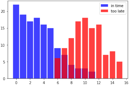
从这些数据中我们可以推断出,如果我们的火车晚点一分钟,赶上转车的概率是 1,因为我们有 19 个成功的案例,没有错过任何一次;也就是说,在 too_late 中没有以 1 为第一个分量的元组。
我们将事件“火车准时到达以赶上转车”表示为 S(成功),将“不幸”事件“火车晚点导致错过转车”表示为 M(错过)。
我们现在可以正式定义概率“在晚点 1 分钟的情况下赶上火车”:
我们利用了 (1, 19) 元组在 in_time 中,并且 too_late 中没有第一个分量为 1 的元组这一事实。
如果我们晚点 6 分钟,赶上前往慕尼黑的转车就变得很关键了。然而,机会仍然有 60%:
相应地,已知我们晚点 6 分钟而错过火车的概率是:
我们可以编写一个“分类器”函数,它将给出赶上转车的概率:
in_time_dict = dict(in_time)
too_late_dict = dict(too_late)

def catch_the_train(min):
    s = in_time_dict.get(min, 0)
    if s == 0:
        return 0
    else:
        m = too_late_dict.get(min, 0)
        return s / (s + m)

for minutes in range(-1, 13):
    print(minutes, catch_the_train(minutes))
Output:
-1 0
0 1.0
1 1.0
2 1.0
3 1.0
4 1.0
5 1.0
6 0.6
7 0.4375
8 0.25
9 0.15
10 0.14285714285714285
11 0.11764705882352941
12 0
一个朴素贝叶斯分类器示例
准备数据
我们将使用一个名为 'person_data.txt' 的文件。它包含 100 个随机的人物数据,包括男性和女性,以及身高、体重和性别标签。
import numpy as np

genders = ["male", "female"]
persons = []
with open("data/person_data.txt") as fh:
    for line in fh:
        persons.append(line.strip().split())

firstnames = {}
heights = {}
for gender in genders:
    firstnames[gender] = [ x[0] for x in persons if x[4]==gender]
    heights[gender] = [ x[2] for x in persons if x[4]==gender]
    heights[gender] = np.array(heights[gender], np.intp) # Changed np.int to np.intp for modern numpy versions

for gender in ("female", "male"):
    print(gender + ":")
    print(firstnames[gender][:10])
    print(heights[gender][:10])
Output:
female:
['Stephanie', 'Cynthia', 'Katherine', 'Elizabeth', 'Carol', 'Christina', 'Beverly', 'Sharon', 'Denise', 'Rebecca']
[149 174 183 138 145 161 179 162 148 196]
male:
['Randy', 'Jessie', 'David', 'Stephen', 'Jerry', 'Billy', 'Earl', 'Todd', 'Martin', 'Kenneth']
[184 175 187 192 204 180 184 174 177 200]
警告: Python 类和朴素贝叶斯类别之间可能会有一些混淆。我们将尽可能明确说明其含义,以避免混淆!
设计特征类
我们现在将为特征定义一个 Python 类 “Feature”,我们稍后将使用它进行分类。
Feature 类需要一个标签,例如“heights”或“firstnames”。如果特征值是数值型的,我们可能希望将它们“分箱”以减少可能的特征值数量。我们人物的身高有一个很大的范围,而我们的朴素贝叶斯类别“male”和“female”只有 50 个测量值。我们将通过将 bin_width 设置为 5,将它们分箱到“130 到 134”、“135 到 139”、“140 到 144”等范围。名字无法分箱,所以 bin_width 将设置为 None。
frequency 方法返回特定特征值或分箱范围的出现次数。
from collections import Counter
import numpy as np

class Feature:
    def __init__(self, data, name=None, bin_width=None):
        self.name = name
        self.bin_width = bin_width
        if bin_width:
            # 确保 bin 的起始点和结束点落在数据范围内,并且是 bin_width 的倍数
            self.min = (min(data) // bin_width) * bin_width
            self.max = ((max(data) + bin_width - 1) // bin_width) * bin_width # 确保包含最大值
            bins = np.arange(self.min, self.max + bin_width, bin_width)
            freq, _ = np.histogram(data, bins=bins) # 使用 bins 参数
            # 创建 freq_dict,键为 bin 的起始值
            self.freq_dict = dict(zip(bins[:-1], freq))
            self.freq_sum = sum(freq)
        else:
            self.freq_dict = dict(Counter(data))
            self.freq_sum = sum(self.freq_dict.values())

    def frequency(self, value):
        if self.bin_width:
            # 对于数值特征,找到其所属的 bin 的起始值
            value_bin_start = (value // self.bin_width) * self.bin_width
            if value_bin_start in self.freq_dict:
                return self.freq_dict[value_bin_start]
            else:
                return 0
        else:
            # 对于非数值特征,直接查找值
            return self.freq_dict.get(value, 0) # 使用 .get() 方法,如果键不存在则返回 0
我们现在将为人员数据集的身高值创建两个特征类 Feature。一个 Feature 类包含朴素贝叶斯类别“male”的身高,另一个包含类别“female”的身高:
fts = {}
for gender in genders:
    fts[gender] = Feature(heights[gender], name=gender, bin_width=5)
    print(gender, fts[gender].freq_dict)
Output:
male {160: 5, 195: 2, 180: 5, 165: 4, 200: 3, 185: 8, 170: 6, 155: 1, 190: 8, 175: 7}
female {160: 8, 130: 1, 165: 11, 135: 1, 170: 7, 140: 0, 175: 2, 145: 3, 180: 4, 150: 5, 185: 0, 155: 7}
频率分布的条形图
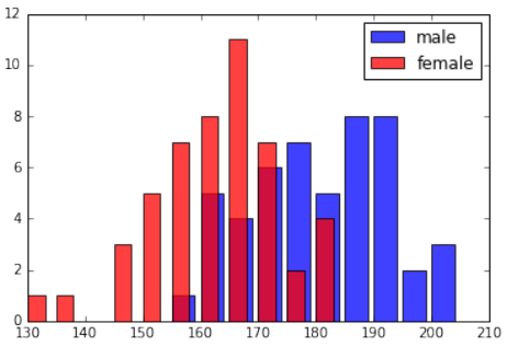
我们打印出了 bin 的频率,但用条形图显示这些值会更好。我们将用以下代码实现这一点:
for gender in genders:
    frequencies = list(fts[gender].freq_dict.items())
    frequencies.sort(key=lambda x: x[0]) # 根据 bin 的起始值排序,以便条形图顺序正确
    X, Y = zip(*frequencies)

    color = "blue" if gender=="male" else "red"
    bar_width = 4 if gender=="male" else 3 # 调整 bar_width 以避免重叠或间隙过大
    plt.bar(X, Y, bar_width, color=color, alpha=0.75, label=gender)
    plt.legend(loc='upper right')
    plt.show()
我们现在必须在 Python 中设计一个朴素贝叶斯类别。我们称之为 NBclass。一个 NBclass 包含一个或多个 Feature 类。NBclass 的名称将存储在 self.name 中。
class NBclass:
    def __init__(self, name, *features):
        self.features = features
        self.name = name

    def probability_value_given_feature(self,
                                        feature_value,
                                        feature):
        """
        p_value_given_feature 返回特征值 'value' 在特征中出现的概率
        对应于 P(d_i | p_j)
        其中 d_i 是特征 i 的特征变量
        """
        if feature.freq_sum == 0:
            return 0
        else:
            return feature.frequency(feature_value) / feature.freq_sum
在以下代码中,我们将创建只有一个特征(即身高特征)的 NBclass。我们将使用我们之前创建的 fts 的 Feature 类:
cls = {}
for gender in genders:
    cls[gender] = NBclass(gender, fts[gender])
创建简单朴素贝叶斯分类器的最后一步是编写一个“分类器”类,它将使用我们的“NBclass”和“Feature”类。
class Classifier:
    def __init__(self, *nbclasses):
        self.nbclasses = nbclasses

    def prob(self, *d, best_only=True):
        nbclasses = self.nbclasses
        probability_list = []
        for nbclass in nbclasses:
            ftrs = nbclass.features
            prob = 1
            for i in range(len(ftrs)):
                prob *= nbclass.probability_value_given_feature(d[i], ftrs[i])
            probability_list.append( (prob, nbclass.name) )

        prob_values = [f[0] for f in probability_list]
        prob_sum = sum(prob_values)
        if prob_sum == 0:
            # 如果所有概率都为0,则平均分配
            number_classes = len(self.nbclasses)
            pl = []
            for prob_element in probability_list:
                pl.append( ((1 / number_classes), prob_element[1]))
            probability_list = pl
        else:
            # 归一化概率
            probability_list = [ (p[0] / prob_sum, p[1]) for p in probability_list]

        if best_only:
            return max(probability_list)
        else:
            return probability_list
我们将创建一个带有一个特征类“height”的分类器。我们用 130 到 220 厘米之间的值检查它。
c = Classifier(cls["male"], cls["female"])
for i in range(130, 220, 5):
    print(i, c.prob(i, best_only=False))
Output:
130 [(0.0, 'male'), (1.0, 'female')]
135 [(0.0, 'male'), (1.0, 'female')]
140 [(0.5, 'male'), (0.5, 'female')]
145 [(0.0, 'male'), (1.0, 'female')]
150 [(0.0, 'male'), (1.0, 'female')]
155 [(0.125, 'male'), (0.875, 'female')]
160 [(0.38461538461538469, 'male'), (0.61538461538461542, 'female')]
165 [(0.26666666666666666, 'male'), (0.73333333333333328, 'female')]
170 [(0.46153846153846162, 'male'), (0.53846153846153855, 'female')]
175 [(0.77777777777777779, 'male'), (0.22222222222222224, 'female')]
180 [(0.55555555555555558, 'male'), (0.44444444444444448, 'female')]
185 [(1.0, 'male'), (0.0, 'female')]
190 [(1.0, 'male'), (0.0, 'female')]
195 [(1.0, 'male'), (0.0, 'female')]
200 [(1.0, 'male'), (0.0, 'female')]
205 [(0.5, 'male'), (0.5, 'female')]
210 [(0.5, 'male'), (0.5, 'female')]
215 [(0.5, 'male'), (0.5, 'female')]
在我们的学习集中,身高在 140 到 144 厘米之间的人(无论是男性还是女性)都没有。这就是为什么我们的分类器不能根据学习数据得出结果,因此得出了五五开的结果。
我们也可以用我们的名字训练一个分类器:
fts = {}
cls = {}
for gender in genders:
    fts_names = Feature(firstnames[gender], name=gender)
    cls[gender] = NBclass(gender, fts_names)
c = Classifier(cls["male"], cls["female"])
testnames = ['Edgar', 'Benjamin', 'Fred', 'Albert', 'Laura',
             'Maria', 'Paula', 'Sharon', 'Jessie']
for name in testnames:
    print(name, c.prob(name))
Output:
Edgar (0.5, 'male')
Benjamin (1.0, 'male')
Fred (1.0, 'male')
Albert (1.0, 'male')
Laura (1.0, 'female')
Maria (1.0, 'female')
Paula (1.0, 'female')
Sharon (1.0, 'female')
Jessie (0.6666666666666667, 'female')
“Jessie”这个名字是一个模糊的名字。每 100 个女孩中大约有 66 个男孩叫这个名字。我们可以从之前的分类结果中得知,名字“Jessie”是“女性”的概率约为三分之二,这是根据我们的“person”数据集计算出来的:
[person for person in persons if person[0] == "Jessie"]
Output:
[['Jessie', 'Morgan', '175', '67.0', 'male'],
['Jessie', 'Bell', '165', '65', 'female'],
['Jessie', 'Washington', '159', '56', 'female'],
['Jessie', 'Davis', '174', '45', 'female'],
['Jessie', 'Johnson', '165', '30.0', 'male'],
['Jessie', 'Thomas', '168', '69', 'female']]
Jessie Washington 身高只有 159 厘米。如果我们查看用身高训练的分类器的结果,我们会发现身高 159 厘米的人是“女性”的可能性为 0.875。那么一个名叫“Jessie”且身高 159 厘米的未知人是女性还是男性呢?
为了回答这个问题,我们将用两个特征类(即身高和名字)训练一个朴素贝叶斯分类器:
cls = {}
for gender in genders:
    fts_heights = Feature(heights[gender], name="heights", bin_width=5)
    fts_names = Feature(firstnames[gender], name="names")
    cls[gender] = NBclass(gender, fts_names, fts_heights)
c = Classifier(cls["male"], cls["female"])
for d in [("Maria", 140), ("Anthony", 200), ("Anthony", 153),
          ("Jessie", 188) , ("Jessie", 159), ("Jessie", 160) ]:
    print(d, c.prob(*d, best_only=False))
Output:
('Maria', 140) [(0.5, 'male'), (0.5, 'female')]
('Anthony', 200) [(1.0, 'male'), (0.0, 'female')]
('Anthony', 153) [(0.5, 'male'), (0.5, 'female')]
('Jessie', 188) [(1.0, 'male'), (0.0, 'female')]
('Jessie', 159) [(0.066666666666666666, 'male'), (0.93333333333333335, 'female')]
('Jessie', 160) [(0.23809523809523817, 'male'), (0.76190476190476197, 'female')]
基本理论
我们上一个示例中的分类器基于贝叶斯定理:
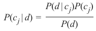
其中:
-
P(\(c_j\)∣d) 是实例 d 属于类别 c_j 的概率,这是我们希望通过分类器计算的结果。
-
P(d∣\(c_j\)) 是在给定类别 c_j 的情况下生成实例 d 的概率。
-
P(\(c_j\)) 是类别 c_j 发生的概率。我们没有在分类器中使用它,因为在我们的示例中,两个类别发生的可能性相等。
-
P(d) 是实例 d 发生的概率。在计算中不需要它,因为它对所有类别都是相同的。
我们之前的示例只使用了一个特征,即“身高”或名字。
可以定义一个具有多个特征的贝叶斯分类器,例如
我们得到以下公式:
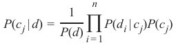
其中 \(\frac{1}{P(d)}\) 仅取决于 的值。这意味着当特征变量的值已知时,它是一个常数。
INTRODUCTORY EXERCISE
Let's set out on a journey by train to create our first
very simple Naive Bayes Classifier. Let us assume
we are in the city of Hamburg and we want to travel
to Munich. We will have to change trains in
Frankfurt am Main. We know from previous train
journeys that our train from Hamburg might be
delayed and the we will not catch our connecting
train in Frankfurt. The probability that we will not be
in time for our connecting train depends on how high
our possible delay will be. The connecting train will
not wait for more than five minutes. Sometimes the
other train is delayed as well.
The following lists 'in_time' (the train from Hamburg arrived in time to catch the connecting train to Munich)
and 'too_late' (connecting train is missed) are data showing the situation over some weeks. The first
component of each tuple shows the minutes the train was late and the second component shows the number of
time this occurred.
# the tuples consist of (delay time of train1, number of times)
# tuples are (minutes, number of times)
in_time = [(0, 22), (1, 19), (2, 17), (3, 18),
(4, 16), (5, 15), (6, 9), (7, 7),
(8, 4), (9, 3), (10, 3), (11, 2)]
too_late = [(6, 6), (7, 9), (8, 12), (9, 17),
(10, 18), (11, 15), (12,16), (13, 7),
(14, 8), (15, 5)]
%matplotlib inline
import matplotlib.pyplot as plt
X, Y = zip(*in_time)
X2, Y2 = zip(*too_late)
bar_width = 0.9
plt.bar(X, Y, bar_width,
color="blue", alpha=0.75, label="in tim
e")
305
bar_width = 0.8
plt.bar(X2, Y2, bar_width, color="red", alpha=0.75, label="too la
te")
plt.legend(loc='upper right')
plt.show()
From this data we can deduce that the probability of catching the connecting train if we are one minute late is
1, because we had 19 successful cases experienced and no misses, i.e. there is no tuple with 1 as the first
component in 'too_late'.
We will denote the event "train arrived in time to catch the connecting train" with S (success) and the 'unlucky'
event "train arrived too late to catch the connecting train" with M (miss)
We can now define the probability "catching the train given that we are 1 minute late" formally:
P(S | 1) = 19 / 19 = 1
We used the fact that the tuple (1, 19) is in 'in_time' and there is no tuple with the first component 1 in
'too_late'
It's getting critical for catching the connecting train to Munich, if we are 6 minutes late. Yet, the chances are
still 60 %:
P(S | 6) = 9 / 9 + 6 = 0.6
Accordingly, the probability for missing the train knowing that we are 6 minutes late is:
P(M | 6) = 6 / 9 + 6 = 0.4
We can write a 'classifier' function, which will give the probability for catching the connecting train:
in_time_dict = dict(in_time)
too_late_dict = dict(too_late)
306
def catch_the_train(min):
s = in_time_dict.get(min, 0)
if s == 0:
return 0
else:
m = too_late_dict.get(min, 0)
return s / (s + m)
for minutes in range(-1, 13):
print(minutes, catch_the_train(minutes))
-1 0
0 1.0
1 1.0
2 1.0
3 1.0
4 1.0
5 1.0
6 0.6
7 0.4375
8 0.25
9 0.15
10 0.14285714285714285
11 0.11764705882352941
12 0
A NAIVE BAYES CLASSIFIER EXAMPLE
GETTING THE DATA READY
We will use a file called 'person_data.txt'. It contains 100 random person data, male and female, with body
sizes, weights and gender tags.
import numpy as np
genders = ["male", "female"]
persons = []
with open("data/person_data.txt") as fh:
for line in fh:
persons.append(line.strip().split())
firstnames = {}
307
heights = {}
for gender in genders:
firstnames[gender] = [ x[0] for x in persons if x[4]==gender]
heights[gender] = [ x[2] for x in persons if x[4]==gender]
heights[gender] = np.array(heights[gender], np.int)
for gender in ("female", "male"):
print(gender + ":")
print(firstnames[gender][:10])
print(heights[gender][:10])
female:
['Stephanie', 'Cynthia', 'Katherine', 'Elizabeth', 'Carol', 'Chris
tina', 'Beverly', 'Sharon', 'Denise', 'Rebecca']
[149 174 183 138 145 161 179 162 148 196]
male:
['Randy', 'Jessie', 'David', 'Stephen', 'Jerry', 'Billy', 'Earl',
'Todd', 'Martin', 'Kenneth']
[184 175 187 192 204 180 184 174 177 200]
Warning: There might be some confusion between a Python class and a Naive Bayes class. We try to avoid it
by saying explicitly what is meant, whenever possible!
DESIGNING A FEATURE CLASS
We will now define a Python class "Feature" for the features, which we will use for classification later.
The Feature class needs a label, e.g. "heights" or "firstnames". If the feature values are numerical we may
want to "bin" them to reduce the number of possible feature values. The heights from our persons have a huge
range and we have only 50 measured values for our Naive Bayes classes "male" and "female". We will bin
them into ranges "130 to 134", "135 to 139", "140 to 144" and so on by setting bin_width to 5. There is no
way of binning the first names, so bin_width will be set to None.
The method frequency returns the number of occurrencies for a certain feature value or a binned range.
from collections import Counter
import numpy as np
class Feature:
def __init__(self, data, name=None, bin_width=None):
self.name = name
self.bin_width = bin_width
if bin_width:
self.min, self.max = min(data), max(data)
308
h,
bins = np.arange((self.min // bin_width) * bin_width,
(self.max // bin_width) * bin_widt
bin_width)
freq, bins = np.histogram(data, bins)
self.freq_dict = dict(zip(bins, freq))
self.freq_sum = sum(freq)
else:
self.freq_dict = dict(Counter(data))
self.freq_sum = sum(self.freq_dict.values())
def frequency(self, value):
if self.bin_width:
value = (value // self.bin_width) * self.bin_width
if value in self.freq_dict:
return self.freq_dict[value]
else:
return 0
We will create now two feature classes Feature for the height values of the person data set. One Feature class
contains the height for the Naive Bayes class "male" and one the heights for the class "female":
fts = {}
for gender in genders:
fts[gender] = Feature(heights[gender], name=gender, bin_widt
h=5)
print(gender, fts[gender].freq_dict)
male {160: 5, 195: 2, 180: 5, 165: 4, 200: 3, 185: 8, 170: 6, 15<br>5: 1, 190: 8, 175: 7}
female {160: 8, 130: 1, 165: 11, 135: 1, 170: 7, 140: 0, 175: 2, 1<br>45: 3, 180: 4, 150: 5, 185: 0, 155: 7}
BAR CHART OF FREQUENCY DISTRIBUTION
We printed out the frequencies of our bins, but it is a lot better to see these values dipicted in a bar chart. We
will do this with the following code:
for gender in genders:
frequencies = list(fts[gender].freq_dict.items())
frequencies.sort(key=lambda x: x[1])
X, Y = zip(*frequencies)
309
color = "blue" if gender=="male" else "red"
bar_width = 4 if gender=="male" else 3
plt.bar(X, Y, bar_width, color=color, alpha=0.75, label=gende
r)
plt.legend(loc='upperplt.show()
right')
We have to design now a Naive Bayes class in Python. We will call it NBclass. An NBclass contains one or
more Feature classes. The name of the NBclass will be stored in self.name.
class NBclass:
def __init__(self, name, *features):
self.features = features
self.name = name
def probability_value_given_feature(self,
feature_value,
feature):
"""
p_value_given_feature returns the probability p
for a feature_value 'value' of the feature to occurr
corresponds to P(d_i | p_j)
where d_i is a feature variable of the feature i
"""
if feature.freq_sum == 0:
return 0
310
else:
return feature.frequency(feature_value) / featur
e.freq_sum
In the following code, we will create NBclasses with one feature, i.e. the height feature. We will use the
Feature classes of fts, which we have previously created:
cls = {}
for gender in genders:
cls[gender] = NBclass(gender, fts[gender])
The final step for creating a simple Naive Bayes classifier consists in writing a class 'Classifier', which will
use our classes 'NBclass' and 'Feature'.
class Classifier:
def __init__(self, *nbclasses):
self.nbclasses = nbclasses
def prob(self, *d, best_only=True):
nbclasses = self.nbclasses
probability_list = []
for nbclass in nbclasses:
ftrs = nbclass.features
prob = 1
for i in range(len(ftrs)):
prob *= nbclass.probability_value_given_featur
e(d[i], ftrs[i])
probability_list.append( (prob, nbclass.name) )
prob_values = [f[0] for f in probability_list]
prob_sum = sum(prob_values)
if prob_sum==0:
number_classes = len(self.nbclasses)
pl = []
for prob_element in probability_list:
pl.append( ((1 / number_classes), prob_elemen
t[1]))
probability_list = pl
else:
probability_list = [ (p[0] / prob_sum, p[1])
for p i
311
nprobability_list]
if best_only:
return max(probability_list)
else:
return probability_list
We will create a classifier with one feature class 'height'. We check it with values between 130 and 220 cm.
c = Classifier(cls["male"], cls["female"])
for i in range(130, 220, 5):
print(i, c.prob(i, best_only=False))
130 [(0.0, 'male'), (1.0, 'female')]
135 [(0.0, 'male'), (1.0, 'female')]
140 [(0.5, 'male'), (0.5, 'female')]
145 [(0.0, 'male'), (1.0, 'female')]
150 [(0.0, 'male'), (1.0, 'female')]
155 [(0.125, 'male'), (0.875, 'female')]
160 [(0.38461538461538469, 'male'), (0.61538461538461542, 'femal
e')]
165 [(0.26666666666666666, 'male'), (0.73333333333333328, 'femal
e')]
170 [(0.46153846153846162, 'male'), (0.53846153846153855, 'femal
e')]
175 [(0.77777777777777779, 'male'), (0.22222222222222224, 'femal
e')]
180 [(0.55555555555555558, 'male'), (0.44444444444444448, 'femal
e')]
185 [(1.0, 'male'), (0.0, 'female')]
190 [(1.0, 'male'), (0.0, 'female')]
195 [(1.0, 'male'), (0.0, 'female')]
200 [(1.0, 'male'), (0.0, 'female')]
205 [(0.5, 'male'), (0.5, 'female')]
210 [(0.5, 'male'), (0.5, 'female')]
215 [(0.5, 'male'), (0.5, 'female')]
There are no persons - neither male nor female - in our learn set, with a body height between 140 and 144.
This is the reason, why our classifier can't base its result on learned data and therefore comes back with a fify-
fifty result.
We can also train a classifier with our firstnames:
fts = {}
cls = {}
312
for gender in genders:
fts_names = Feature(firstnames[gender], name=gender)
cls[gender] = NBclass(gender, fts_names)
c = Classifier(cls["male"], cls["female"])
testnames = ['Edgar', 'Benjamin', 'Fred', 'Albert', 'Laura',
'Maria', 'Paula', 'Sharon', 'Jessie']
for name in testnames:
print(name, c.prob(name))
Edgar (0.5, 'male')
Benjamin (1.0, 'male')
Fred (1.0, 'male')
Albert (1.0, 'male')
Laura (1.0, 'female')
Maria (1.0, 'female')
Paula (1.0, 'female')
Sharon (1.0, 'female')
Jessie (0.6666666666666667, 'female')
The name "Jessie" is an ambiguous name. There are about 66 boys per 100 girls with this name. We can learn
from the previous classification results that the probability for the name "Jessie" being "female" is about two-
thirds, which is calculated from our data set "person":
[person for person in persons if person[0] == "Jessie"]
Output:[['Jessie', 'Morgan', '175', '67.0', 'male'],
['Jessie', 'Bell', '165', '65', 'female'],
['Jessie', 'Washington', '159', '56', 'female'],
['Jessie', 'Davis', '174', '45', 'female'],
['Jessie', 'Johnson', '165', '30.0', 'male'],
['Jessie', 'Thomas', '168', '69', 'female']]
Jessie Washington is only 159 cm tall. If we have a look at the results of our Classifier, trained with heights,
we see that the likelihood for a person 159 cm tall of being "female" is 0.875. So what about an unknown
person called "Jessie" and being 159 cm tall? Is this person female or male?
To answer this question, we will train an Naive Bayes classifier with two feature classes, i.e. heights and
firstnames:
cls = {}
for gender in genders:
fts_heights = Feature(heights[gender], name="heights", bin_wid
th=5)
313
fts_names = Feature(firstnames[gender], name="names")
cls[gender] = NBclass(gender, fts_names, fts_heights)
c = Classifier(cls["male"], cls["female"])
for d in [("Maria", 140), ("Anthony", 200), ("Anthony", 153),
("Jessie", 188) , ("Jessie", 159), ("Jessie", 160) ]:
print(d, c.prob(*d, best_only=False))
('Maria', 140) [(0.5, 'male'), (0.5, 'female')]
('Anthony', 200) [(1.0, 'male'), (0.0, 'female')]
('Anthony', 153) [(0.5, 'male'), (0.5, 'female')]
('Jessie', 188) [(1.0, 'male'), (0.0, 'female')]
('Jessie', 159) [(0.066666666666666666, 'male'), (0.93333333333333
335, 'female')]
('Jessie', 160) [(0.23809523809523817, 'male'), (0.761904761904761
97, 'female')]
THE UNDERLYING THEORY
Our classifier from the previous example is based on the Bayes theorem:
P(d | c j)P(c j)
P(cj | d) =
P(d)
where
• P(c j | d) is the probability of instance d being in class c_j, it is the result we want to calculate
with our classifier
• P(d | cj) is the probability of generating the instance d, if the class c j is given
• P(c j) is the probability for the occurrence of class cj We didn't use it in our classifiers, because
both classes in our example have been equally likely.
• P(d) is the probability for the occurrence of an instance d It's not needed in the calculation,
because it is the same for all classes.
We had used only one feature in our previous examples, i.e. the 'height' or the name.
It's possible to define a Bayes Classifier with multiple features, e.g. d = (d 1, d2, . . . , dn)
314
We get the following formula:
n
1
P(c j | d) =
∏ P(di | cj)P(c j)
P(d)i = 1
1
P ( d )
is only depending on the values of d1, d 2, . . . dn. This means that it is a constant as the values of the
feature variables are known.
In [ ]: