机器学习
决策树是一种监督机器学习(这意味着您在训练数据中说明了输入和相应的输出)模型,它根据特定参数连续地分割数据。决策树可以由两个实体解释:决策节点和叶子。叶子是决策或最终结果,而决策节点是数据被分割的地方。
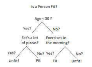
我们可以用上面的二叉树来解释一个决策树的例子。假设您想根据一个人的年龄、饮食习惯和体育活动等信息来预测他是否健康。这里的决策节点是“年龄是多少?”、“他锻炼吗?”和“他经常吃披萨吗?”这样的问题。而叶子则是“健康”或“不健康”这样的结果。在这种情况下,这是一个二元分类问题(是/否类型的问题)。决策树主要有两种类型:
-
分类树(是/否类型)
我们上面看到的就是一个分类树的例子,其中结果是一个变量,如“健康”或“不健康”。这里的决策变量是分类变量。
-
回归树(连续数据类型)
在这里,决策或结果变量是连续的,例如一个数字,如 123。
工作原理
现在我们知道了什么是决策树,接下来我们将了解它是如何在内部工作的。有许多算法可以构建决策树,但其中最好的一种叫做 ID3 算法。ID3 代表迭代二分器 3(Iterative Dichotomiser 3)。在讨论 ID3 算法之前,我们先了解几个定义。
熵
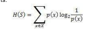
熵,也称为香农熵,对于有限集 S 用 H(S) 表示,是衡量数据中不确定性或随机性的量。
直观地说,它告诉我们某个事件的可预测性。例如,考虑抛硬币,正面朝上的概率是 0.5,反面朝上的概率是 0.5。在这里,熵是最高的,因为无法确定结果是什么。另一方面,考虑一个两面都是正面的硬币,这种事件的熵可以完美预测,因为我们事先知道它总是正面朝上。换句话说,这个事件没有随机性,因此它的熵为零。特别是,较低的值意味着较少的不确定性,而较高的值意味着高度不确定性。
信息增益
信息增益也称为Kullback-Leibler 散度,对于集合 S 用 IG(S,A) 表示,是决定了特定属性 A 之后,熵的有效变化。它衡量的是熵相对于自变量的相对变化。
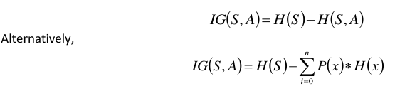
其中 IG(S,A) 是通过应用特征 A 获得的信息增益。 H(S) 是整个集合的熵,而第二项计算应用特征 A 后的熵,其中 P(xi) 是事件 xi 的概率。
让我们通过一个例子来理解这一点。考虑在 14 天内收集到的一段数据,其中特征是 Outlook(天气)、Temperature(温度)、Humidity(湿度)、Wind(风),结果变量是当天是否打高尔夫球。现在,我们的任务是构建一个预测模型,该模型输入以上 4 个参数并预测当天是否会打高尔夫球。我们将使用 ID3 算法构建一个决策树来完成此任务。
| Day | Outlook | Temperature | Humidity | Wind | Play Golf |
| :-- | :--------- | :---------- | :------- | :----- | :-------- |
| D1 | Sunny | Hot | High | Weak | No |
| D2 | Sunny | Hot | High | Strong | No |
| D3 | Overcast | Hot | High | Weak | Yes |
| D4 | Rain | Mild | High | Weak | Yes |
| D5 | R1ain | Cool | Normal | Weak | Yes |
| D6 | Rain | Cool | Normal | Strong | No |
| D7 | Overcast | Cool | Normal | Strong | Yes |
| D8 | Sunny | Mild | High | Weak | No |
| D9 | Sunny | Cool | Normal | Weak | Yes |
| D10 | Rain | Mild | Normal | Weak | Yes |
| D11 | Sunny | Mild | Normal | Strong | Yes |
| D12 | Overcast | Mild | High | Strong | Yes |
| D13 | Overcast | Hot | Normal | Weak | Yes |
| D14 | Rain | Mild | High | Strong | No |
Introduction Decision Trees are a type of Supervised Machine Learning (that is you explain what
the input is and what the corresponding output is in the training data) where the data is continuously
split according to a certain parameter. The tree can be explained by two entities, namely decision
nodes and leaves. The leaves are the decisions or the final outcomes. And the decision nodes are where
the data is split.
An example of a decision tree can be explained using above binary tree. Let’s say you want to predict whether a person if fit given their infomation like age,eating habit,and physical activity etc. The decision nodes here are questions like ‘What’s the age?’, ‘Does he exercise?’, and ‘Does he eat a lot of
pizzas’? And the leaves, which are outcomes like either ‘fit’, or ‘unfit’. In this case this was a binary
classification problem (a yes no type problem). There are two main types of Decision Trees:
1. Classification trees (Yes/No types)
What we have seen above is an example of classification tree, where the outcome was a variable like
‘fit’ or ‘unfit’. Here the decision variable is Categorical.
2. Regression trees (Continuous data types)
Here the decision or the outcome variable is Continuous, e.g. a number like 123. Working Now that we
know what a Decision Tree is, we’ll see how it works internally. There are many algorithms out there
which construct Decision Trees, but one of the best is called as ID3 Algorithm. ID3 Stands for Iterative
Dichotomiser 3. Before discussing the ID3 algorithm, we’ll go through few definitions. Entropy Entropy,
also called as Shannon Entropy is denoted by H(S) for a finite set S, is the measure of the amount of
uncertainty or randomness in data.
Intuitively, it tells us about the predictability of a certain event. Example, consider a coin toss whose
probability of heads is 0.5 and probability of tails is 0.5. Here the entropy is the highest possible, since
there’s no way of determining what the outcome might be. Alternatively, consider a coin which has
heads on both the sides, the entropy of such an event can be predicted perfectly since we know
beforehand that it’ll always be heads. In other words, this event has no randomness hence it’s entropy
is zero. In particular, lower values imply less uncertainty while higher values imply high
uncertainty. Information Gain Information gain is also called as Kullback-Leibler divergence denoted by
IG(S,A) for a set S is the effective change in entropy after deciding on a particular attribute A. It
measures the relative change in entropy with respect to the independent variables
Alternatively,
IG S , A H S H S , A
IG S , A H S n
P x H x
i 0
where IG(S, A) is the information gain by applying feature A. H(S) is the Entropy of the entire set, while
the second term calculates the Entropy after applying the feature A, where P(x) is the probability of
event x. Let’s understand this with the help of an example Consider a piece of data collected over the
course of 14 days where the features are Outlook, Temperature, Humidity, Wind and the outcome
variable is whether Golf was played on the day. Now, our job is to build a predictive model which takes
in above 4 parameters and predicts whether Golf will be played on the day. We’ll build a decision tree
to do that using ID3 algorithm.
Day
Outlook
Temperature
Humidity
Wind
Play Golf
D1
Sunny
Hot
High
Weak
No
D2
Sunny
Hot
High
Strong
No
D3
Overcast
Hot
High
Weak
Yes
25
D4
Rain
Mild
D5
Rain
Cool
D6
Rain
Cool
D7
Overcast
Cool
D8
Sunny
Mild
D9
Sunny
Cool
D10
Rain
Mild
D11
Sunny
Mild
D12
Overcast
Mild
D13
Overcast
Hot
D14
Rain
Mild
High
Weak
Yes
Normal
Weak
Yes
Normal
Strong
No
Normal
Strong
Yes
High
Weak
No
Normal
Weak
Yes
Normal
Weak
Yes
Normal
Strong
Yes
High
Strong
Yes
Normal
Weak
Yes
High
Strong
No