机器学习
-
逻辑回归是另一种监督学习算法,用于解决分类问题。在分类问题中,我们的因变量是二元或离散格式,例如 0 或 1。
-
逻辑回归算法处理类别变量,例如 0 或 1、是或否、真或假、垃圾邮件或非垃圾邮件等。
-
它是一种基于概率概念的预测分析算法。
-
逻辑回归是一种回归类型,但它在使用方式上与线性回归算法不同。
-
逻辑回归使用S 型函数或逻辑函数,这是一个复杂的成本函数。这个 S 型函数用于对逻辑回归中的数据进行建模。该函数可以表示为:
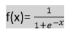
f(x)=1+e−x1
其中:
- f(x) = 输出值在 0 和 1 之间。
- x = 函数的输入。
- e = 自然对数的底数。
-
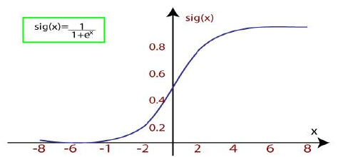
当我们向函数提供输入值(数据)时,它会给出如下所示的 S 形曲线:
-
它使用阈值的概念,高于阈值的值四舍五入为 1,低于阈值的值四舍五入为 0。
-
逻辑回归有三种类型:
- 二元(0/1,通过/失败)
- 多类别(猫、狗、狮子)
- 序数(低、中、高)
机器学习中的线性回归(重复内容,但在原文本中再次出现,故此处也翻译)
线性回归是最简单和最流行的机器学习算法之一。它是一种用于预测分析的统计方法。线性回归对连续/实数或数值变量进行预测,例如销售额、薪资、年龄、产品价格等。
线性回归算法显示因变量(y)与一个或多个自变量(x)之间的线性关系,因此被称为线性回归。由于线性回归显示线性关系,这意味着它发现因变量的值如何根据自变量的值而变化。
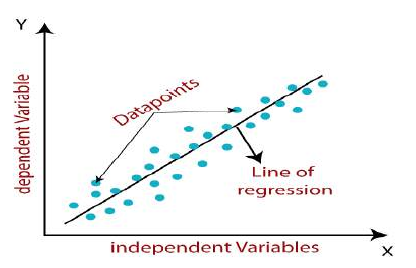
线性回归模型提供一条倾斜的直线,表示变量之间的关系。请看下图:
从数学上,我们可以将线性回归表示为:
y=a0+a1x+ϵ
其中:
- Y = 因变量(目标变量)
- X = 自变量(预测变量)
- a0 = 直线的截距(提供额外的自由度)
- a1 = 线性回归系数(每个输入值的比例因子)
- ϵ = 随机误差
x 和 y 变量的值是线性回归模型表示的训练数据集。
线性回归的类型
线性回归可以进一步分为两种类型的算法:
- 简单线性回归: 如果使用单个自变量来预测数值因变量的值,那么这种线性回归算法称为简单线性回归。
- 多元线性回归: 如果使用多个自变量来预测数值因变量的值,那么这种线性回归算法称为多元线性回归。
线性回归线:
显示因变量和自变量之间关系的线性直线称为回归线。回归线可以显示两种类型的关系:
-
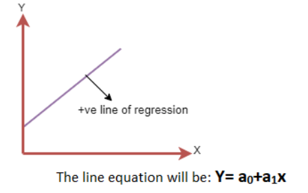
正线性关系:
如果因变量在 Y 轴上增加,自变量在 X 轴上增加,则这种关系被称为正线性关系。
-
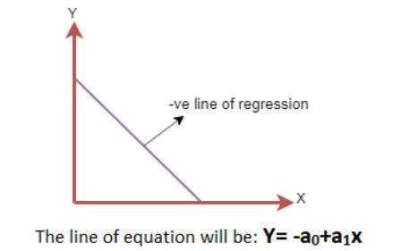
负线性关系:
如果因变量在 Y 轴上减少,自变量在 X 轴上增加,则这种关系被称为负线性关系。
寻找最佳拟合线:
在使用线性回归时,我们的主要目标是找到最佳拟合线,这意味着预测值和实际值之间的误差应该最小化。最佳拟合线的误差最小。
权重或直线系数 (a0,a1) 的不同值会给出不同的回归线,因此我们需要计算 a0 和 a1 的最佳值来找到最佳拟合线,为此我们使用成本函数。
成本函数
- 权重或直线系数 (a0,a1) 的不同值会给出不同的回归线,成本函数用于估计最佳拟合线的系数的值。
- 成本函数优化回归系数或权重。它衡量线性回归模型的性能。
- 我们可以使用成本函数来找到映射函数(将输入变量映射到输出变量)的准确性。这个映射函数也称为假设函数。
对于线性回归,我们使用均方误差(MSE)成本函数,它是预测值和实际值之间发生的平方误差的平均值。它可以写成:
MSE=N1i=1∑N(Yi−(a1Xi+a0))2
对于上述线性方程,MSE 可以计算为:
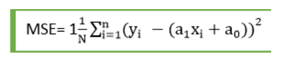
其中:
- N = 观测值的总数
- Yi = 实际值
- = 预测值。
残差:实际值和预测值之间的距离称为残差。如果观测点距离回归线较远,则残差会很高,因此成本函数也会很高。如果散点靠近回归线,则残差会很小,因此成本函数也会很小。
梯度下降:
- 梯度下降用于通过计算成本函数的梯度来最小化 MSE。
- 回归模型使用梯度下降来通过减少成本函数来更新直线的系数。
- 这是通过随机选择系数的值,然后迭代更新这些值以达到最小成本函数来完成的。
模型性能:
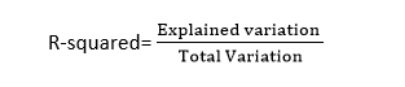
拟合优度决定了回归线如何拟合观测集。从各种模型中找到最佳模型的过程称为优化。它可以通过以下方法实现:
- R 方方法:
- R 方是一种确定拟合优度的统计方法。
- 它衡量因变量和自变量之间关系的强度,范围为 0-100%。
- R 方值越高,表示预测值和实际值之间的差异越小,因此代表一个好的模型。
- 它也称为决定系数,或多元回归的复决定系数。
- 它可以根据以下公式计算:
线性回归的假设
以下是线性回归的一些重要假设。这些是在构建线性回归模型时的一些正式检查,确保从给定数据集中获得最佳可能结果。
- 特征和目标之间的线性关系: 线性回归假设因变量和自变量之间存在线性关系。
- 特征之间小或无多重共线性: 多重共线性意味着自变量之间存在高度相关性。由于多重共线性,可能难以找到预测变量和目标变量之间的真实关系。或者我们可以说,很难确定哪个预测变量正在影响目标变量,哪个没有。因此,模型假设特征或自变量之间只有很小或没有多重共线性。
- 同方差性假设: 同方差性是指对于自变量的所有值,误差项都相同的情况。在同方差性下,散点图中不应有明显的数据分布模式。
- 误差项的正态分布: 线性回归假设误差项应遵循正态分布模式。如果误差项不呈正态分布,则置信区间将变得过宽或过窄,这可能导致难以找到系数。 这可以使用 Q-Q 图进行检查。如果图显示一条没有偏差的直线,则意味着误差呈正态分布。
- 无自相关: 线性回归模型假设误差项中没有自相关。如果误差项中存在任何相关性,则会大大降低模型的准确性。自相关通常发生在残差错误之间存在依赖关系时。
机器学习中的简单线性回归
简单线性回归是一种回归算法类型,它模拟因变量与单个自变量之间的关系。简单线性回归模型显示的关系是线性的或倾斜的直线,因此称为简单线性回归。
简单线性回归的关键点是因变量必须是连续/实数值。然而,自变量可以在连续或类别值上测量。
简单线性回归算法主要有两个目标:
- 建模两个变量之间的关系。例如收入与支出、经验与薪资之间的关系等。
- 预测新的观测值。例如根据温度进行天气预报、公司在一年内的投资收益等。
简单线性回归模型:
简单线性回归模型可以使用以下方程表示:
y=a0+a1x+ϵ
其中:
- a0 = 回归线的截距(可以通过将 得到)
- a1 = 回归线的斜率,表示直线是上升还是下降。
- ϵ = 误差项。(对于一个好的模型,它将可以忽略不计)
o
Logistic regression is another supervised learning algorithm which is used to solve the classification
problems. In classification problems, we have dependent variables in a binary or discrete format such as 0
or 1.
o
Logistic regression algorithm works with the categorical variable such as 0 or 1, Yes or No, True or False,
Spam or not spam, etc.
o
It is a predictive analysis algorithm which works on the concept of probability.
o
Logistic regression is a type of regression, but it is different from the linear regression algorithm in the
term how they are used.
o
Logistic regression uses sigmoid function or logistic function which is a complex cost function. This
sigmoid function is used to model the data in logistic regression. The function can be represented as:
34
o
o
o
f(x)= Output between the 0 and 1 value.
x= input to the function
e= base of natural logarithm.
When we provide the input values (data) to the function, it gives the S-curve as follows:
o
It uses the concept of threshold levels, values above the threshold level are rounded up to 1, and values
below the threshold level are rounded up to 0.
There are three types of logistic regression:
o Binary(0/1, pass/fail)
o
Multi(cats, dogs, lions)
o
Ordinal(low, medium, high)
Linear Regression in Machine Learning
Linear regression is one of the easiest and most popular Machine Learning algorithms. It is a statistical method that
is used for predictive analysis. Linear regression makes predictions for continuous/real or numeric variables such
as sales, salary, age, product price, etc.
Linear regression algorithm shows a linear relationship between a dependent and one or more independent
variables, hence called as linear regression. Since linear regression shows the linear relationship, which means it
finds how the value of the dependent variable is changing according to the value of the independent variable.
The linear regression model provides a sloped straight line representing the relationship between the variables.
Consider the below image:
35
Mathematically, we can represent a linear regression as:
y= a0+a1x+ ε
Here,
Y= Dependent Variable (Target Variable)
X= Independent Variable (predictor Variable)
a0= intercept of the line (Gives an additional degree of freedom)
a1 = Linear regression coefficient (scale factor to each input value).
ε = random error
The values for x and y variables are training datasets for Linear Regression model representation.
Types of Linear Regression
Linear regression can be further divided into two types of the algorithm:
o Simple Linear Regression:
If a single independent variable is used to predict the value of a numerical dependent variable, then such a
Linear Regression algorithm is called Simple Linear Regression.
o
Multiple Linear regression:
If more than one independent variable is used to predict the value of a numerical dependent variable, then
such a Linear Regression algorithm is called Multiple Linear Regression.
Linear Regression Line:
A linear line showing the relationship between the dependent and independent variables is called a regression line.
A regression line can show two types of relationship:
o Positive Linear Relationship:
If the dependent variable increases on the Y-axis and independent variable increases on X-axis, then such a
relationship is termed as a Positive linear relationship.
36
o
Negative Linear Relationship:
If the dependent variable decreases on the Y-axis and independent variable increases on the X-axis, then
such a relationship is called a negative linear relationship.
Finding the best fit
line:
When working with linear regression, our main goal is to find the best fit line that means the error between
predicted values and actual values should be minimized. The best fit line will have the least error.
The different values for weights or the coefficient of lines (a0, a1) gives a different line of regression, so we
need to calculate the best values for a0 and a1 to find the best fit line, so to calculate this we use cost function.
Cost function-
o The different values for weights or coefficient of lines (a0, a1) gives the different line of regression, and the
cost function is used to estimate the values of the coefficient for the best fit line.
o
o
Cost function optimizes the regression coefficients or weights. It measures how a linear regression model
is performing.
We can use the cost function to find the accuracy of the mapping function, which maps the input variable
to the output variable. This mapping function is also known as Hypothesis function.
For Linear Regression, we use the Mean Squared Error (MSE) cost function, which is the average of
squared error occurred between the predicted values and actual values. It can be written as:
37
For the above linear equation, MSE can be calculated as:
Where,
N=Total number of observation
Yi = Actual value
(a1xi+a0)= Predicted value.
Residuals: The distance between the actual value and predicted values is called residual. If the observed points are
far from the regression line, then the residual will be high, and so cost function will high. If the scatter points are
close to the regression line, then the residual will be small and hence the cost function.
Gradient Descent:
o Gradient descent is used to minimize the MSE by calculating the gradient of the cost function.
o
A regression model uses gradient descent to update the coefficients of the line by reducing the cost
function.
o
It is done by a random selection of values of coefficient and then iteratively update the values to reach the
minimum cost function.
Model Performance:
The Goodness of fit determines how the line of regression fits the set of observations. The process of
finding the best model out of various models is called optimization. It can be achieved by below method:
1. R-squared method:
o R-squared is a statistical method that determines the goodness of fit.
o
It measures the strength of the relationship between the dependent and independent variables on a scale of
0-100%.
o
The high value of R-square determines the less difference between the predicted values and actual values
and hence represents a good model.
o
It is also called a coefficient of determination, or coefficient of multiple determination for multiple
regression.
o
It can be calculated from the below formula:
Assumptions of Linear Regression
Below are some important assumptions of Linear Regression. These are some formal checks while building a
Linear Regression model, which ensures to get the best possible result from the given dataset.
o
Linear relationship between the features and target:
Linear regression assumes the linear relationship between the dependent and independent variables.
o
Small or no multicollinearity between the features:
Multicollinearity means high-correlation between the independent variables. Due to multicollinearity, it
may difficult to find the true relationship between the predictors and target variables. Or we can say, it is
difficult to determine which predictor variable is affecting the target variable and which is not. So, the
model assumes either little or no multicollinearity between the features or independent variables.
o
Homoscedasticity Assumption:
Homoscedasticity is a situation when the error term is the same for all the values of independent variables.
With homoscedasticity, there should be no clear pattern distribution of data in the scatter plot.
o
Normal distribution of error terms:
Linear regression assumes that the error term should follow the normal distribution pattern. If error terms
are not normally distributed, then confidence intervals will become either too wide or too narrow, which
may cause difficulties in finding coefficients.
It can be checked using the q-q plot. If the plot shows a straight line without any deviation, which means
the error is normally distributed.
o
No autocorrelations:
The linear regression model assumes no autocorrelation in error terms. If there will be any correlation in
the error term, then it will drastically reduce the accuracy of the model. Autocorrelation usually occurs if
there is a dependency between residual errors.
Simple Linear Regression in Machine Learning
Simple Linear Regression is a type of Regression algorithms that models the relationship between a dependent
variable and a single independent variable. The relationship shown by a Simple Linear Regression model is linear or
a sloped straight line, hence it is called Simple Linear Regression.
The key point in Simple Linear Regression is that the dependent variable must be a continuous/real value.
However, the independent variable can be measured on continuous or categorical values.
Simple Linear regression algorithm has mainly two objectives:
o
Model the relationship between the two variables. Such as the relationship between Income and
expenditure, experience and Salary, etc.
o
Forecasting new observations. Such as Weather forecasting according to temperature, Revenue of a
company according to the investments in a year, etc.
Simple Linear Regression Model:
The Simple Linear Regression model can be represented using the below equation:
y= a0+a1x+ ε
Where,
a0= It is the intercept of the Regression line (can be obtained putting x=0)
a1= It is the slope of the regression line, which tells whether the line is increasing or decreasing.
ε = The error term. (For a good model it will be negligible)