机器学习Python教程
线性可分数据集
正如我们在机器学习教程的上一章中所示,仅由一个感知器组成的神经网络足以分离我们的示例类别。当然,我们精心设计了这些类别以使其奏效。然而,许多类别的集群是无法通过这种方式分离的。我们将看一些其他示例,并讨论无法分离类别的情况。
我们的类别是线性可分的。线性可分性在欧几里得几何中是有意义的。如果平面中存在至少一条直线,使得一个类的所有点都在该直线的一侧,而另一个类的所有点都在该直线的另一侧,那么两个点集(或类别)就被称为线性可分。
更正式地说:
如果两个数据簇(类别)可以通过线性方程形式的决策边界进行分离,它们就被称为线性可分:
否则,即如果不存在这样的决策边界,这两个类别被称为线性不可分。在这种情况下,我们不能使用简单的神经网络。
用于 AND 函数的感知器
在我们的下一个示例中,我们将用 Python 编程一个实现逻辑“与”功能的神经网络。它针对两个输入定义如下:
|
输入1 |
输入2 |
输出 |
|
0 |
0 |
0 |
|
0 |
1 |
0 |
|
1 |
0 |
0 |
|
1 |
1 |
1 |
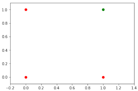
我们在上一章中了解到,一个包含一个感知器和两个输入值的神经网络可以被解释为一个决策边界,即一条划分两个类别的直线。我们想在示例中分类的两个类别如下所示:
import matplotlib.pyplot as plt
import numpy as np

fig, ax = plt.subplots()
xmin, xmax = -0.2, 1.4
X = np.arange(xmin, xmax, 0.1)

# 红色点代表输出 0
ax.scatter(0, 0, color="r")
ax.scatter(0, 1, color="r")
ax.scatter(1, 0, color="r")
# 绿色点代表输出 1
ax.scatter(1, 1, color="g")

ax.set_xlim([xmin, xmax])
ax.set_ylim([-0.1, 1.1])

# m = -1
# ax.plot(X, m * X + 1.2, label="decision boundary") # 这行被注释掉了
plt.plot()
输出:[]
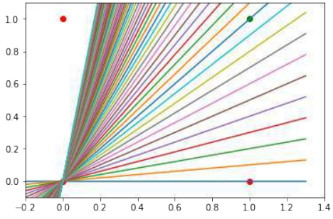
我们还发现,这种原始的神经网络只能创建通过原点的直线。因此,像这样的分隔线:
import matplotlib.pyplot as plt
import numpy as np

fig, ax = plt.subplots()
xmin, xmax = -0.2, 1.4
X = np.arange(xmin, xmax, 0.1)

ax.set_xlim([xmin, xmax])
ax.set_ylim([-0.1, 1.1])

m = -1 # 初始斜率值,但后面循环会被覆盖
for m_val in np.arange(0, 6, 0.1): # 循环尝试不同的斜率值
    ax.plot(X, m_val * X, color='gray', linestyle='--', alpha=0.5) # 绘制通过原点的直线

# 绘制数据点
ax.scatter(0, 0, color="r")
ax.scatter(0, 1, color="r")
ax.scatter(1, 0, color="r")
ax.scatter(1, 1, color="g")

plt.plot()
输出:[]
我们可以看到,这些通过原点的直线都不能用作决策边界。
我们需要一条形如以下形式的直线:
y = m . x + c
其中截距 c 不等于 0。
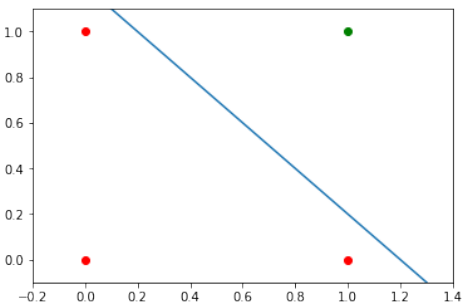
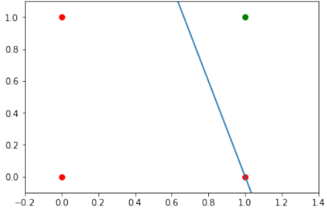
例如,直线
y = −x + 1.2
可以用作我们问题的分隔线:
import matplotlib.pyplot as plt
import numpy as np

fig, ax = plt.subplots()
xmin, xmax = -0.2, 1.4
X = np.arange(xmin, xmax, 0.1)

ax.scatter(0, 0, color="r")
ax.scatter(0, 1, color="r")
ax.scatter(1, 0, color="r")
ax.scatter(1, 1, color="g")

ax.set_xlim([xmin, xmax])
ax.set_ylim([-0.1, 1.1])

m, c = -1, 1.2 # 斜率和截距
ax.plot(X, m * X + c, color='blue', linewidth=2, label='y = -x + 1.2') # 绘制直线
ax.legend() # 显示图例
plt.plot()
输出:[]
现在的问题是,我们是否可以通过对网络模型进行微小修改来找到解决方案?或者换句话说:我们能否创建一个能够定义任意决策边界的感知器?
解决方案在于添加一个偏置节点。
带有偏置的单感知器
一个带有两个输入值和一个偏置的感知器对应于一条一般的直线。借助偏置值 b,我们可以训练感知器来确定一个具有非零截距 c 的决策边界。
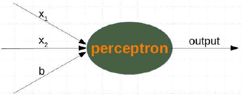
虽然输入值可以改变,但偏置值始终保持不变。只有偏置节点的权重可以被调整。
现在,感知器的线性方程包含一个偏置:
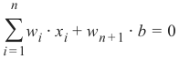
在我们的例子中,它看起来像这样:
![]()
这等价于:
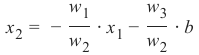
这意味着:

且
import numpy as np
from collections import Counter

class Perceptron:
    def __init__(self,
                 weights,
                 bias=1, # 偏置值
                 learning_rate=0.3):
        self.weights = np.array(weights)
        self.bias = bias
        self.learning_rate = learning_rate

    @staticmethod
    def unit_step_function(x):
        if x <= 0: # 修正:对于 AND 函数,0 应该输出 0
            return 0
        else:
            return 1

    def __call__(self, in_data):
        # 将偏置值添加到输入数据中
        in_data = np.concatenate((in_data, [self.bias]))
        result = self.weights @ in_data # 使用矩阵乘法
        return Perceptron.unit_step_function(result)

    def adjust(self,
               target_result,
               in_data):
        if not isinstance(in_data, np.ndarray): # 修正:使用 isinstance
            in_data = np.array(in_data)

        calculated_result = self(in_data) # 调用 __call__ 方法计算结果
        error = target_result - calculated_result

        if error != 0:
            # 将偏置值添加到输入数据中,以便计算权重校正
            in_data_with_bias = np.concatenate((in_data, [self.bias]))
            correction = error * in_data_with_bias * self.learning_rate
            self.weights += correction

    def evaluate(self, data, labels):
        evaluation = Counter()
        for sample, label in zip(data, labels):
            result = self(sample) # 预测
            if result == label:
                evaluation["correct"] += 1
            else:
                evaluation["wrong"] += 1
        return evaluation
我们假设上述包含 Perceptron 类的 Python 代码已存储在您当前的工作目录中,文件名为 perceptrons.py。
import numpy as np
# from perceptrons import Perceptron # 假设 Perceptron 类已定义或导入

def labelled_samples(n):
    for _ in range(n):
        s = np.random.randint(0, 2, (2,)) # 随机生成 0 或 1 的输入
        # AND 逻辑:只有当两个输入都为 1 时,输出为 1
        yield (s, 1) if s[0] == 1 and s[1] == 1 else (s, 0)

p = Perceptron(weights=[0.3, 0.3, 0.3], # 初始权重,包括偏置项的权重
               learning_rate=0.2)

# 训练感知器
for in_data, label in labelled_samples(30): # 使用 30 个样本进行训练
    p.adjust(label, in_data)

# 测试感知器
test_data, test_labels = list(zip(*labelled_samples(30))) # 生成 30 个测试样本
evaluation = p.evaluate(test_data, test_labels)
print(evaluation)
Counter({'correct': 30})
import matplotlib.pyplot as plt
import numpy as np

fig, ax = plt.subplots()
xmin, xmax = -0.2, 1.4
X = np.arange(xmin, xmax, 0.1)

# 绘制数据点
ax.scatter(0, 0, color="r")
ax.scatter(0, 1, color="r")
ax.scatter(1, 0, color="r")
ax.scatter(1, 1, color="g")

ax.set_xlim([xmin, xmax])
ax.set_ylim([-0.1, 1.1])

# 使用训练后的感知器权重计算决策边界的斜率和截距
m = -p.weights[0] / p.weights[1]
c = -p.weights[2] / p.weights[1] * p.bias # 修正:截距 c 也要考虑偏置值 b
print(m, c)
ax.plot(X, m * X + c, color='blue', linewidth=2, label='Decision Boundary') # 绘制决策边界
ax.legend()
plt.plot()
plt.show()
-3.0000000000000004 3.0000000000000013
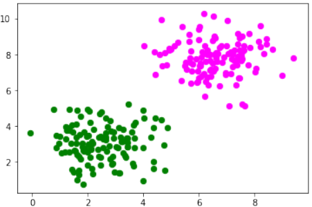
我们将创建另一个需要偏置节点才能分离的线性可分数据集示例。我们将使用 sklearn.datasets 中的 make_blobs 函数:
from sklearn.datasets import make_blobs
import numpy as np # 确保 numpy 被导入

n_samples = 250
samples, labels = make_blobs(n_samples=n_samples,
                             centers=([2.5, 3], [6.7, 7.9]), # 两个聚类的中心点
                             random_state=0) # 固定随机状态以保证可复现性
让我们可视化之前创建的数据:
import matplotlib.pyplot as plt
# colours = ('green', 'magenta', 'blue', 'cyan', 'yellow', 'red') # 原始代码有太多颜色,这里只用2个
colours = ('green', 'magenta') # 两个类别只需要两种颜色
fig, ax = plt.subplots()
for n_class in range(2): # 只有两个类别 (0 和 1)
    ax.scatter(samples[labels==n_class][:, 0], samples[labels==n_class][:, 1],
               c=colours[n_class], s=40, label=str(n_class))

ax.legend() # 显示图例
plt.show()
# from perceptrons import Perceptron # 假设 Perceptron 类已定义或导入
import numpy as np
from collections import Counter
import matplotlib.pyplot as plt # 确保导入 matplotlib.pyplot

n_learn_data = int(n_samples * 0.8) # 80% 的可用数据点作为训练数据
learn_data, test_data = samples[:n_learn_data], samples[n_learn_data:] # 修正:这里应该是 n_learn_data:
learn_labels, test_labels = labels[:n_learn_data], labels[n_learn_data:] # 修正:这里应该是 n_learn_data:

p = Perceptron(weights=[0.3, 0.3, 0.3], # 初始权重
               learning_rate=0.8)

# 训练感知器
for sample, label in zip(learn_data, learn_labels):
    p.adjust(label, sample)

evaluation = p.evaluate(learn_data, learn_labels)
print(evaluation)
Counter({'correct': 200})
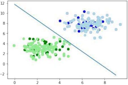
让我们可视化决策边界:
import matplotlib.pyplot as plt
import numpy as np # 确保导入 numpy

fig, ax = plt.subplots()

# 绘制训练数据
colours = ('green', 'blue') # 训练数据颜色
for n_class in range(2):
    ax.scatter(learn_data[learn_labels==n_class][:, 0],
               learn_data[learn_labels==n_class][:, 1],
               c=colours[n_class], s=40, label=f"Train Class {n_class}")

# 绘制测试数据
colours = ('lightgreen', 'lightblue') # 测试数据颜色
for n_class in range(2):
    ax.scatter(test_data[test_labels==n_class][:, 0],
               test_data[test_labels==n_class][:, 1],
               c=colours[n_class], s=40, label=f"Test Class {n_class}")

# 确保 X 轴范围覆盖所有数据
x_min_plot = np.min(samples[:,0]) - 1
x_max_plot = np.max(samples[:,0]) + 1
X_plot = np.arange(x_min_plot, x_max_plot, 0.1) # 绘制直线的 X 范围

# 计算决策边界的斜率和截距
m = -p.weights[0] / p.weights[1]
c = -p.weights[2] / p.weights[1] * p.bias # 考虑到偏置值

print(m, c)
ax.plot(X_plot, m * X_plot + c, color='red', linewidth=2, label="Decision Boundary") # 绘制决策边界
ax.legend() # 显示图例
plt.grid(True) # 添加网格
plt.show()
-1.5513529034664024 11.736643489707035
在下一节中,我们将介绍神经网络中的 XOR 问题。它是最简单的非线性可分神经网络示例。它可以通过额外的神经元层来解决,这层被称为隐藏层。
神经网络的 XOR 问题
XOR(异或)函数由以下真值表定义:
|
输入1 |
输入2 |
XOR 输出 |
|
0 |
0 |
0 |
|
0 |
1 |
1 |
|
1 |
0 |
1 |
|
1 |
1 |
0 |
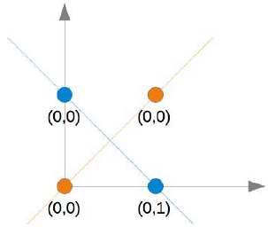
这个问题无法用简单的神经网络解决,正如我们在下图中看到的那样:
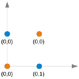
(图片:一个二维坐标系,X轴为Input1,Y轴为Input2。点(0,0)和(1,1)是橙色,点(0,1)和(1,0)是蓝色。图中有多条直线,试图分开这些点,但都失败了。)
无论你选择哪条直线,你都无法成功地将蓝色点放在一边而橙色点放在另一边。这在下图中有所展示。橙色点在橙色线上。这意味着这不能作为分隔线。如果我们平行移动这条线——无论哪个方向,总会有两个橙色点和一个蓝色点在同一侧,而另一侧只有一个蓝色点。如果我们将橙色线非平行移动,则两侧都会有一个蓝色点和一个橙色点,除非直线穿过一个橙色点。因此,没有办法用一条直线来分隔这些点。
为了解决这个问题,我们需要引入一种新型的神经网络,即带有隐藏层的网络。隐藏层允许网络重组或重新排列输入数据。
我们只需要一个包含两个神经元的隐藏层。一个神经元像一个 AND 门一样工作,另一个像一个 OR 门一样工作。当 OR 门激活而 AND 门不激活时,输出将“激活”。
正如我们已经提到的,我们无法找到一条将橙色点与蓝色点分开的线。但它们可以被两条线分开,例如下图中所示的 L1 和 L2:
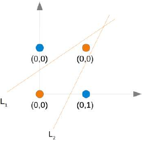
(图片:一个二维坐标系,点(0,0)和(1,1)是橙色,点(0,1)和(1,0)是蓝色。图中画了两条直线,L1和L2,它们共同将橙色点与蓝色点区分开。)
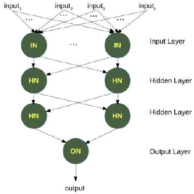
为了解决这个问题,我们需要一个如下所示的网络,即带有隐藏层 N1 和 N2:
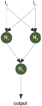
(图片:一个神经网络的结构图。左侧是输入层,两个输入节点。中间是隐藏层,包含两个神经元 N1 和 N2。右侧是输出层,一个神经元 N3。输入节点与 N1 和 N2 连接,N1 和 N2 又与 N3 连接。)
神经元 N1 将确定一条线,例如 L1;神经元 N2 将确定另一条线 L2。N3 最终将解决我们的问题:
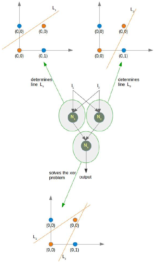
(图片:一个更详细的神经网络结构图,显示了每个神经元(N1, N2, N3)如何根据输入和内部权重进行计算,并最终推导出 XOR 问题的逻辑分离,通过两个线 L1 和 L2 的组合作用来实现复杂边界。)
在 Python 中实现这一点必须等到我们机器学习教程的下一章。
练习
练习 1
我们可以将逻辑 AND 扩展到 0 到 1 之间的浮点值,如下所示:
|
Input1 |
Input2 |
Output |
|
x1 < 0.5 |
x2 < 0.5 |
0 |
|
x1 < 0.5 |
x2 >= 0.5 |
0 |
|
x1 >= 0.5 |
x2 < 0.5 |
0 |
|
x1 >= 0.5 |
x2 >= 0.5 |
1 |
尝试只用一个感知器训练一个神经网络。为什么它不起作用?
练习 2
如果 \(x_1\) < 0.5,一个点属于类别 0;如果 ,则属于类别 1。训练一个只用一个感知器的网络来分类任意点。你对决策边界有什么看法?输入值 $$x_2$$ 呢?
练习答案
练习 1 答案
# from perceptrons import Perceptron # 假设 Perceptron 类已定义或导入
import numpy as np
from collections import Counter

p = Perceptron(weights=[0.3, 0.3, 0.3],
               bias=1,
               learning_rate=0.2)

def labelled_samples(n):
    for _ in range(n):
        s = np.random.random((2,)) # 生成 0 到 1 之间的浮点数
        # 扩展的 AND 逻辑
        yield (s, 1) if s[0] >= 0.5 and s[1] >= 0.5 else (s, 0)

# 训练感知器
for in_data, label in labelled_samples(30):
    p.adjust(label, in_data)

# 测试感知器
test_data, test_labels = list(zip(*labelled_samples(60)))
evaluation = p.evaluate(test_data, test_labels)
print(evaluation)
Counter({'correct': 32, 'wrong': 28}) # 结果可能因随机性而异
最容易看出为什么它不起作用的方法是可视化数据。
import matplotlib.pyplot as plt
import numpy as np

# 从测试数据中分离出类别 1(绿色)和类别 0(红色)的点
ones = [test_data[i] for i in range(len(test_data)) if test_labels[i] == 1]
zeroes = [test_data[i] for i in range(len(test_data)) if test_labels[i] == 0]

fig, ax = plt.subplots()
xmin, xmax = -0.2, 1.2

# 绘制类别 1 的点
if ones: # 检查列表是否为空
    X_ones, Y_ones = zip(*ones)
    ax.scatter(X_ones, Y_ones, color="g", label="Output 1")
# 绘制类别 0 的点
if zeroes: # 检查列表是否为空
    X_zeroes, Y_zeroes = zip(*zeroes)
    ax.scatter(X_zeroes, Y_zeroes, color="r", label="Output 0")

ax.set_xlim([xmin, xmax])
ax.set_ylim([-0.1, 1.1])

# 计算决策边界的斜率和截距
# 假设 p.weights[1] 不是零
if p.weights[1] != 0:
    c = -p.weights[2] / p.weights[1] * p.bias
    m = -p.weights[0] / p.weights[1]
else: # 如果 w2 为零,直线是垂直的
    c = -p.weights[2] / p.weights[0] * p.bias # 此时 c 代表 x 截距
    m = np.inf # 无穷大斜率

X_plot = np.arange(xmin, xmax, 0.1)

# 根据 m 是否为无穷大绘制直线
if np.isinf(m):
    # 垂直线
    ax.axvline(x=-p.weights[2] / p.weights[0] * p.bias, color='blue', linestyle='--', label="Decision Boundary (vertical)")
else:
    # 非垂直线
    ax.plot(X_plot, m * X_plot + c, color='blue', linewidth=2, label="Decision Boundary")

ax.legend()
plt.show()
输出:[<matplotlib.lines.Line2D at ...>] (或其他 matplotlib 对象)
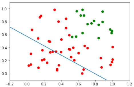
我们可以看到绿色点和红色点不能被一条直线分开。这与我们之前讨论的 XOR 问题有相似之处,因为它们都不是线性可分的。
练习 2 答案
# from perceptrons import Perceptron # 假设 Perceptron 类已定义或导入
import numpy as np
from collections import Counter

def labelled_samples(n):
    for _ in range(n):
        s = np.random.random((2,))
        # 分类规则:x1 < 0.5 属于类别 0,x1 >= 0.5 属于类别 1
        yield (s, 0) if s[0] < 0.5 else (s, 1)

p = Perceptron(weights=[0.3, 0.3, 0.3], # 初始权重
               learning_rate=0.4)

# 训练感知器
for in_data, label in labelled_samples(300):
    p.adjust(label, in_data)

# 测试感知器
test_data, test_labels = list(zip(*labelled_samples(500)))
print(p.weights)
evaluation = p.evaluate(test_data, test_labels) # 修正:这里需要将 evaluation 赋值
print(evaluation)
[ 2.03831116 -0.1785671  -0.9       ]
Counter({'correct': 489, 'wrong': 11}) # 结果可能因随机性而异
import matplotlib.pyplot as plt
import numpy as np

# 从测试数据中分离出类别 1(绿色)和类别 0(红色)的点
ones = [test_data[i] for i in range(len(test_data)) if test_labels[i] == 1]
zeroes = [test_data[i] for i in range(len(test_data)) if test_labels[i] == 0]

fig, ax = plt.subplots()
xmin, xmax = -0.2, 1.2

# 绘制类别 1 的点
if ones:
    X_ones, Y_ones = zip(*ones)
    ax.scatter(X_ones, Y_ones, color="g", label="Class 1")
# 绘制类别 0 的点
if zeroes:
    X_zeroes, Y_zeroes = zip(*zeroes)
    ax.scatter(X_zeroes, Y_zeroes, color="r", label="Class 0")

ax.set_xlim([xmin, xmax])
ax.set_ylim([-0.1, 1.1])

# 计算决策边界的斜率和截距
# 假设 p.weights[1] 不是零
if p.weights[1] != 0:
    c = -p.weights[2] / p.weights[1] * p.bias
    m = -p.weights[0] / p.weights[1]
else: # 如果 w2 为零,直线是垂直的
    c = -p.weights[2] / p.weights[0] * p.bias # 此时 c 代表 x 截距
    m = np.inf # 无穷大斜率

X_plot = np.arange(xmin, xmax, 0.01) # 增加点密度使直线更平滑

# 根据 m 是否为无穷大绘制直线
if np.isinf(m):
    # 垂直线
    ax.axvline(x=-p.weights[2] / p.weights[0] * p.bias, color='blue', linewidth=2, label="Decision Boundary (vertical)")
else:
    # 非垂直线
    ax.plot(X_plot, m * X_plot + c, color='blue', linewidth=2, label="Decision Boundary")

ax.legend()
plt.show()
输出:[<matplotlib.lines.Line2D at ...>] (或其他 matplotlib 对象)
print(p.weights, m)
(array([ 2.03831116, -0.1785671 , -0.9 ]), 11.414819026) # 结果可能因随机性而异
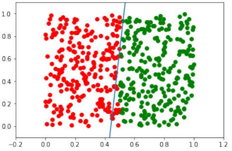
在这种情况下,斜率 m 将变得越来越大。
这个练习的结果显示,决策边界是一条近似垂直的直线。这是因为分类规则主要依赖于输入值 $$x_1$$。当 \(x_1\) < 0.5 时,点属于类别 0,当 时,点属于类别 1。这意味着分隔线应该大致在 处。
对于输入值 \(x_2\),它对分类的影响非常小,因为决策边界几乎是垂直的。这意味着无论 \(x_2\) 的值是多少,只要 \(x_1\) 满足条件,点就会被正确分类。这反映在训练后的权重中,与 \(x_2\) 相关的权重(即 p.weights[1])的绝对值通常会很小,从而导致决策边界的斜率非常大(接近垂直)。
这些练习帮助我们理解了感知器在处理线性可分数据方面的能力和局限性。如果数据不是线性可分的,或者需要更复杂的决策边界,我们就需要更高级的神经网络结构,例如引入隐藏层。
您是否想深入了解隐藏层如何解决 XOR 问题,或者探索其他类型的神经网络?
LINEARLY SEPARABLE DATA SETS
As we have shown in the previous chapter of our tutorial on machine
learning, a neural network consisting of only one perceptron was enough to
separate our example classes. Of course, we carefully designed these
classes to make it work. There are many clusters of classes, for whichit will
not work. We are going to have a look at some other examples and will
discuss cases where it will not be possible to separate the classes.
Our classes have been linearly separable. Linear separability make sense
in Euclidean geometry. Two sets of points (or classes) are called linearly
separable, if at least one straight line in the plane exists so that all the
points of one class are on one side of the line and all the points of the other
class are on the other side.
More formally:
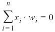
If two data clusters (classes) can be separated by a decision boundary in the
form of a linear equation
n
∑ x i ⋅ wi = 0
i =1
they are called linearly separable.
Otherwise, i.e. if such a decision boundary does not exist, the two classes are called linearly inseparable. In
this case, we cannot use a simple neural network.
PERCEPTRON FOR THE AND FUNCTION
In our next example we will program a Neural Network in Python which implements the logical "And"
function. It is defined for two inputs in the following way:
Input1
Input2
Output
0
0
0
0
1
0
1
0
0
117
Input1
Input2
Output
1
1
1
We learned in the previous chapter that a neural network with one perceptron and two input values can be
interpreted as a decision boundary, i.e. straight line dividing two classes. The two classes we want to classify
in our example look like this:
import matplotlib.pyplot as plt
import numpy as np
fig, ax = plt.subplots()
xmin, xmax = -0.2, 1.4
X = np.arange(xmin, xmax, 0.1)
ax.scatter(0, 0, color="r")
ax.scatter(0, 1, color="r")
ax.scatter(1, 0, color="r")
ax.scatter(1, 1, color="g")
ax.set_xlim([xmin, xmax])
ax.set_ylim([-0.1, 1.1])
m = -1
#ax.plot(X, m * X + 1.2, label="decision boundary")
plt.plot()
Output:[]
We also found out that such a primitive neural network is only capable of creating straight lines going through
the origin. So dividing lines like this:
118
import matplotlib.pyplot as plt
import numpy as np
fig, ax = plt.subplots()
xmin, xmax = -0.2, 1.4
X = np.arange(xmin, xmax, 0.1)
ax.set_xlim([xmin, xmax])
ax.set_ylim([-0.1, 1.1])
m = -1
for m in np.arange(0, 6, 0.1):
ax.plot(X, m * X )
ax.scatter(0, 0, color="r")
ax.scatter(0, 1, color="r")
ax.scatter(1, 0, color="r")
ax.scatter(1, 1, color="g")
plt.plot()
Output:[]
We can see that none of these straight lines can be used as decision boundary nor any other lines going
through the origin.
We need a line
y = m ⋅ x + c
where the intercept c is not equal to 0.
For example the line
y = − x + 1.2
119
could be used as a separating line for our problem:
import matplotlib.pyplot as plt
import numpy as np
fig, ax = plt.subplots()
xmin, xmax = -0.2, 1.4
X = np.arange(xmin, xmax, 0.1)
ax.scatter(0, 0, color="r")
ax.scatter(0, 1, color="r")
ax.scatter(1, 0, color="r")
ax.scatter(1, 1, color="g")
ax.set_xlim([xmin, xmax])
ax.set_ylim([-0.1, 1.1])
m, c = -1, 1.2
ax.plot(X, m * X + c )
plt.plot()
Output:[]
The question now is whether we can find a solution with minor modifications of our network model? Or in
other words: Can we create a perceptron capable of defining arbitrary decision boundaries?
The solution consists in the addition of a bias node.
SINGLE PERCEPTRON WITH A BIAS
A perceptron with two input values and a bias corresponds to a general straight line. With the aid of the bias
value b we can train the perceptron to determine a decision boundary with a non zero intercept c .
120
While the input values can change, a bias value always remains constant. Only the weight of the bias node can
be adapted.
Now, the linear equation for a perceptron contains a bias:
n
∑ w i ⋅ x i + w n + 1 ⋅ b = 0
i =1
In our case it looks like this:
w 1 ⋅ x 1 + w 2 ⋅ x 2 + w 3 ⋅ b = 0
this is equivalent with
w1
w 3
x2 = −
⋅ x 1 −
⋅ b
w2
w 2
This means:
w1
m = −
w2
and
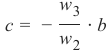
w3
c = −
⋅ b
w 2
import numpy as np
from collections import Counter
class Perceptron:
def __init__(self,
121
weights,
bias=1,
learning_rate=0.3):
"""
'weights' can be a numpy array, list or a tuple with the
actual values of the weights. The number of input values
is indirectly defined by the length of 'weights'
"""
self.weights = np.array(weights)
self.bias = bias
self.learning_rate = learning_rate
@staticmethod
def unit_step_function(x):
if x <= 0:
return 0
else:
return 1
def __call__(self, in_data):
in_data = np.concatenate( (in_data, [self.bias]) )
result = self.weights @ in_data
return Perceptron.unit_step_function(result)
def adjust(self,
target_result,
in_data):
if type(in_data) != np.ndarray:
in_data = np.array(in_data) #
calculated_result = self(in_data)
error = target_result - calculated_result
if error != 0:
in_data = np.concatenate( (in_data, [self.bias]) )
correction = error * in_data * self.learning_rate
self.weights += correction
def evaluate(self, data, labels):
evaluation = Counter()
for sample, label in zip(data, labels):
result = self(sample) # predict
if result == label:
evaluation["correct"] += 1
else:
evaluation["wrong"] += 1
return evaluation
122
We assume that the above Python code with the Perceptron class is stored in your current working directory
under the name 'perceptrons.py'.
import numpy as np
from perceptrons import Perceptron
def labelled_samples:
for _ in range:
s = np.random.randint(0, 2, (2,))
yield (s, 1) if s[0] == 1 and s[1] == 1 else (s, 0)
p = Perceptron(weights=[0.3, 0.3, 0.3],
learning_rate=0.2)
for in_data, label in labelled_samples(30):
p.adjust(label,
in_data)
test_data, test_labels = list(zip(*labelled_samples(30)))
evaluation = p.evaluate(test_data, test_labels)
print(evaluation)
Counter({'correct': 30})
import matplotlib.pyplot as plt
import numpy as np
fig, ax = plt.subplots()
xmin, xmax = -0.2, 1.4
X = np.arange(xmin, xmax, 0.1)
ax.scatter(0, 0, color="r")
ax.scatter(0, 1, color="r")
ax.scatter(1, 0, color="r")
ax.scatter(1, 1, color="g")
ax.set_xlim([xmin, xmax])
ax.set_ylim([-0.1, 1.1])
m = -p.weights[0] / p.weights[1]
c = -p.weights[2] / p.weights[1]
print(m, c)
ax.plot(X, m * X + c )
plt.plot()
123
-3.0000000000000004Output:[]
3.0000000000000013
We will create another example with linearly separable data sets, which need a bias node to be separable. We
will use the make_blobs function from sklearn.datasets :
from sklearn.datasets import make_blobs
n_samples = 250
samples, labels = make_blobs(n_samples=n_samples,
centers=([2.5, 3], [6.7, 7.9]),
random_state=0)
Let us visualize the previously created data:
import matplotlib.pyplot as plt
colours = ('green', 'magenta', 'blue', 'cyan', 'yellow', 'red')
fig, ax = plt.subplots()
for n_class in range(2):
ax.scatter(samples[labels==n_class][:, 0], samples[labels==n_c
lass][:, 1],
c=colours[n_class], s=40, label=str(n_class))
124
n_learn_data = int(n_samples * 0.8) # 80 % of available data point
s
learn_data, test_data = samples[:n_learn_data], samples[-n_learn_d
ata:]
learn_labels, test_labels = labels[:n_learn_data], labels[-n_lear
n_data:]
from perceptrons import Perceptron
p = Perceptron(weights=[0.3, 0.3, 0.3],
learning_rate=0.8)
for sample, label in zip(learn_data, learn_labels):
p.adjust(label,
sample)
evaluation = p.evaluate(learn_data, learn_labels)
print(evaluation)
Counter({'correct': 200})
Let us visualize the decision boundary:
import matplotlib.pyplot as plt
fig, ax = plt.subplots()
# plotting learn data
colours = ('green', 'blue')
125
for n_class in range(2):
ax.scatter(learn_data[learn_labels==n_class][:, 0],
learn_data[learn_labels==n_class][:, 1],
c=colours[n_class], s=40, label=str(n_class))
# plotting test data
colours = ('lightgreen', 'lightblue')
for n_class in range(2):
ax.scatter(test_data[test_labels==n_class][:, 0],
test_data[test_labels==n_class][:, 1],
c=colours[n_class], s=40, label=str(n_class))
X = np.arange(np.max(samples[:,0]))
m = -p.weights[0] / p.weights[1]
c = -p.weights[2] / p.weights[1]
print(m, c)
ax.plot(X, m * X + c )
plt.plot()
plt.show()
-1.5513529034664024 11.736643489707035
In the following section, we will introduce the XOR problem for neural networks. It is the simplest example of
a non linearly separable neural network. It can be solved with an additional layer of neurons, which is called a
hidden layer.
126
THE XOR PROBLEM FOR NEURAL NETWORKS
The XOR (exclusive or) function is defined by the following truth table:
Input1
Input2
XOR Output
0
0
0
0
1
1
1
0
1
1
1
0
This problem can't be solved with a simple neural network, as we can see in the following diagram:
No matter which straight line you choose, you will never succeed in having the blue points on one side and the
orange points on the other side. This is shown in the following figure. The orange points are on the orange
line. This means that this cannot be a dividing line. If we move this line parallel - no matter which direction,
there will be always two orange and one blue point on one side and only one blue point on the other side. If we
move the orange line in a non parallel way, there will be one blue and one orange point on either side, except
if the line goes through an orange point. So there is no way for a single straight line separating those points.
127
To solve this problem, we need to introduce a new type of neural networks, a network with so-called hidden
layers. A hidden layer allows the network to reorganize or rearrange the input data.
We will need only one hidden layer with two neurons. One works like an AND gate and the other one like an
OR gate. The output will "fire", when the OR gate fires and the AND gate doesn't.
As we had already mentioned, we cannot find a line which separates the orange points from the blue points.
But they can be separated by two lines, e.g. L1 and L2 in the following diagram:
128
To solve this problem, we need a network of the following kind, i.e with a hidden layer N1 and N2
The neuron N1 will determine one line, e.g. L1 and the neuron N2 will determine the other line L2. N3 will
finally solve our problem:
129
The implementation of this in Python has to wait until the next chapter of our tutorial on machine learning.
130
EXERCISES
EXERCISE 1
We could extend the logical AND to float values between 0 and 1 in the following way:
Input1
Input2
Output
x1 < 0.5
x2 < 0.5
0
x1 < 0.5
x2 >= 0.5
0
x1 >= 0.5
x2 < 0.5
0
x1 >= 0.5
x2 >= 0.5
1
Try to train a neural network with only one perceptron. Why doesn't it work?
EXERCISE 2
A point belongs to a class 0, if x 1 < 0.5 and belongs to class 1, if x 1 >= 0.5. Train a network with one
perceptron to classify arbitrary points. What can you say about the dicision boundary? What about the input
values x 2
SOLUTIONS TO THE EXERCISES
SOLUTION TO THE 1. EXERCISE
from perceptrons import Perceptron
p = Perceptron(weights=[0.3, 0.3, 0.3],
bias=1,
learning_rate=0.2)
def labelled_samples:
for _ in range:
s = np.random.random((2,))
yield (s, 1) if s[0] >= 0.5 and s[1] >= 0.5 else (s, 0)
for in_data, label in labelled_samples(30):
p.adjust(label,
131
in_data)
test_data, test_labels = list(zip(*labelled_samples(60)))
evaluation = p.evaluate(test_data, test_labels)
print(evaluation)
Counter({'correct': 32, 'wrong': 28})
The easiest way to see, why it doesn't work, is to visualize the data.
import matplotlib.pyplot as plt
import numpy as np
ones = [test_data[i] for i in range(len(test_data)) if test_label
s[i] == 1]
zeroes = [test_data[i] for i in range(len(test_data)) if test_labe
ls[i] == 0]
fig, ax = plt.subplots()
xmin, xmax = -0.2, 1.2
X, Y = list(zip(*ones))
ax.scatter(X, Y, color="g")
X, Y = list(zip(*zeroes))
ax.scatter(X, Y, color="r")
ax.set_xlim([xmin, xmax])
ax.set_ylim([-0.1, 1.1])
c = -p.weights[2] / p.weights[1]
m = -p.weights[0] / p.weights[1]
X = np.arange(xmin, xmax, 0.1)
ax.plot(X, m * X + c, label="decision boundary")
132
Output:[<matplotlib.lines.Line2D at 0x7fabe8bfbf90>]
We can see that the green points and the red points are not separable by one straight line.
SOLUTION TO THE 2ND EXERCISE
from perceptrons import Perceptron
import numpy as np
from collections import Counter
def labelled_samples:
for _ in range:
s = np.random.random((2,))
yield (s, 0) if s[0] < 0.5 else (s, 1)
p = Perceptron(weights=[0.3, 0.3, 0.3],
learning_rate=0.4)
for in_data, label in labelled_samples(300):
p.adjust(label,
in_data)
test_data, test_labels = list(zip(*labelled_samples(500)))
print(p.weights)
p.evaluate(test_data, test_labels)
133
[ 2.03831116 -0.1785671
-0.9
]
Output:Counter({'correct': 489, 'wrong': 11})
import matplotlib.pyplot as plt
import numpy as np
ones = [test_data[i] for i in range(len(test_data)) if test_label
s[i] == 1]
zeroes = [test_data[i] for i in range(len(test_data)) if test_labe
ls[i] == 0]
fig, ax = plt.subplots()
xmin, xmax = -0.2, 1.2
X, Y = list(zip(*ones))
ax.scatter(X, Y, color="g")
X, Y = list(zip(*zeroes))
ax.scatter(X, Y, color="r")
ax.set_xlim([xmin, xmax])
ax.set_ylim([-0.1, 1.1])
c = -p.weights[2] / p.weights[1]
m = -p.weights[0] / p.weights[1]
X = np.arange(xmin, xmax, 0.1)
ax.plot(X, m * X + c, label="decision boundary")
Output:[<matplotlib.lines.Line2D at 0x7fabe8bc89d0>]
p.weights, m
Outputarray([ 2.03831116, -0.1785671 , -0.9
425487)
]), 11.414819026
134
The slope m will have to get larger and larger in situations like this.