从分界线到神经网络(From Dividing Lines to Neural Networks)
章节大纲
-
引言
 在本教程的这一章中,我们将开发一个简单的神经网络。该网络能够分离在二维特征空间中可通过直线分离的两个类别。
直线分离
在我们开始编写一个简单的神经网络程序之前,我们先来发展一个不同的概念。我们想要寻找能够将平面上的两点或两类分开的直线。我们目前只关注通过原点的直线。我们将在本教程的后面部分探讨更一般的直线。
你可以想象,你有两个属性来描述一个可食用的物体,比如水果:“甜度”和“酸度”。
我们可以用二维空间中的点来描述这一点。x 轴用于表示甜度值,y 轴相应地用于表示酸度值。现在想象一下,我们在这个空间中有两种水果作为点,例如,橙子在位置 (3.5, 1.8),柠檬在 (1.1, 3.9)。
我们可以定义分割线来区分哪些点更像柠檬,哪些点更像橙子。
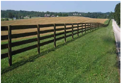
在下面的图中,我们展示了一个柠檬和一个橙子。绿线将这两个点分开了。我们假设所有其他柠檬都在这条线上方,所有橙子都在这条线下方。
(图片:一个二维坐标系,X轴为甜度,Y轴为酸度。有一个橙色的点代表橙子,一个黄色的点代表柠檬。一条绿线穿过原点,将橙子和柠檬分开。)
绿线由以下方程定义:
y=mx
其中:
m 是线的斜率或梯度,x 是函数的自变量。
斜率

这意味着如果满足以下条件,点
 在这条线上:
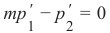
以下 Python 程序绘制了描述上述情况的图:
Pythonimport matplotlib.pyplot as plt import numpy as np X = np.arange(0, 7) fig, ax = plt.subplots() ax.plot(3.5, 1.8, "or", # 修正:颜色使用 darkorange color="darkorange", markersize=15) ax.plot(1.1, 3.9, "oy", markersize=15) point_on_line = (4, 4.5) # ax.plot(1.1, 3.9, "oy", markersize=15) # 这一行是重复的,可以删除 # calculate gradient: m = point_on_line[1] / point_on_line[0] ax.plot(X, m * X, "g-", linewidth=3) plt.show()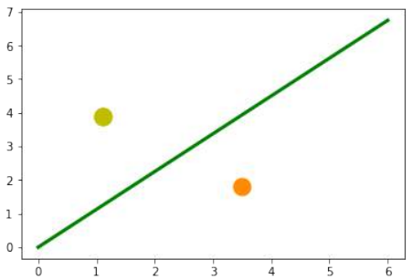
很明显,如果
 不等于0,则点
  不在线上。我们想知道更多。我们想知道一个点是在直线上方还是下方。
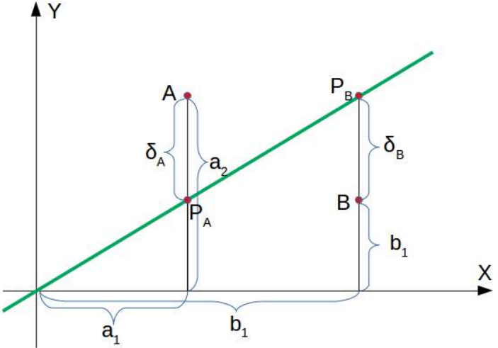
如果点
 在这条线下方,则必须存在
  ,使得点
,使得点  会在这条线上。
这意味着
可以重新排列为
最终,我们得到了一个点在线下方的判别标准。由于
 是正数,
是正数, 是正数。
是正数。“点在线上方”的推理是类似的:如果点
 在线上方,则必须存在
  ,使得点
,使得点 会在这条线上。
这意味着
可以重新排列为
总而言之,我们可以说:点
 位于:
位于:-
直线下方,如果
 > 0
> 0 -
直线上,如果
 = 0
= 0 -
直线上方,如果
 < 0
< 0
现在我们可以在我们的水果上验证这一点。柠檬的坐标是 (1.1, 3.9),橙子的坐标是 (3.5, 1.8)。我们用来定义分隔直线的线上的点的值是 (4, 4.5)。所以 m 是 4.5 除以 4。
Pythonlemon = (1.1, 3.9) orange = (3.5, 1.8) m = 4.5 / 4 # 检查橙子是否在线下方, # 期望值为正: print(orange[0] * m - orange[1]) # 检查柠檬是否在线上方, # 期望值为负: print(lemon[0] * m - lemon[1])2.1375 -2.6624999999999996我们没有使用数学公式或方法计算绿线,而是凭视觉判断任意确定的。我们也可以选择其他线。
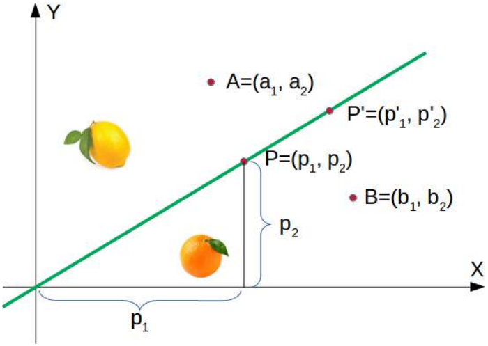
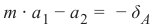
以下 Python 程序计算并渲染了一堆直线。所有直线都通过原点,即点 (0, 0)。红色的线完全不能用于分隔这两种水果,因为在这些情况下,柠檬和橙子都在直线的同一侧。然而,很明显,即使是绿色的线,如果水果数量不止这两种,也可能不太有用。有些柠檬可能更甜,有些橙子可能相当酸。
Pythonimport numpy as np import matplotlib.pyplot as plt def create_distance_function(a, b, c): """ 0 = ax + by + c """ def distance(x, y): """ 返回元组 (d, pos) d 是距离 如果 pos == -1 点在线下方, 0 在线上,+1 在线上方 """ nom = a * x + b * y + c if nom == 0: pos = 0 elif (nom < 0 and b < 0) or (nom > 0 and b > 0): pos = -1 else: pos = 1 return (np.absolute(nom) / np.sqrt(a ** 2 + b ** 2), pos) # 修正:pos应该在元组中 return distance orange = (4.5, 1.8) # 修正:使用更合适的橙子坐标,例如原始文本中的 (3.5, 1.8) 更符合图示 lemon = (1.1, 3.9) fruits_coords = [orange, lemon] fig, ax = plt.subplots() ax.set_xlabel("sweetness") ax.set_ylabel("sourness") x_min, x_max = -1, 7 y_min, y_max = -1, 8 ax.set_xlim([x_min, x_max]) ax.set_ylim([y_min, y_max]) X = np.arange(x_min, x_max, 0.1) step = 0.05 for x_val in np.arange(0, 1 + step, step): # 修正:变量名改为 x_val 避免与全局 X 冲突 slope = np.tan(np.arccos(x_val)) dist4line1 = create_distance_function(slope, -1, 0) # 直线方程为 slope * x - y = 0 Y = slope * X results = [] for point in fruits_coords: results.append(dist4line1(*point)) # 解包点坐标 if (results[0][1] != results[1][1]): # 如果两个水果在直线的不同侧 ax.plot(X, Y, "g-", linewidth=0.8, alpha=0.9) else: # 如果在同一侧 ax.plot(X, Y, "r-", linewidth=0.8, alpha=0.9) size = 10 for (index, (x, y)) in enumerate(fruits_coords): if index == 0: ax.plot(x, y, "o", color="darkorange", markersize=size) else: ax.plot(x, y, "oy", markersize=size) plt.show()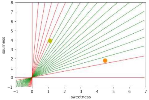
基本上,我们已经根据我们的分割线进行了一次分类。即使几乎没有人会这样描述。
很容易想象我们有更多具有略微不同酸甜度的柠檬和橙子。这意味着我们有一类柠檬(
class1)和一类橙子(class2)。这在以下图中有所描述。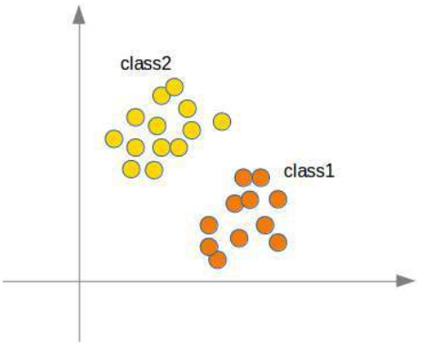
(图片:一个二维坐标系,X轴为甜度,Y轴为酸度。散布着橙色的点代表橙子,黄色的点代表柠檬,形成两个大致分开的簇。一条绿线穿过两个簇之间。)
我们将通过一个 Python 程序来“种植”橙子和柠檬。我们将通过在具有定义中心点和半径的圆形内随机创建点来创建这两个类。以下 Python 代码将创建这些类:
Pythonimport numpy as np import matplotlib.pyplot as plt def points_within_circle(radius, center=(0, 0), number_of_points=100): center_x, center_y = center r = radius * np.sqrt(np.random.random((number_of_points,))) theta = np.random.random((number_of_points,)) * 2 * np.pi x = center_x + r * np.cos(theta) y = center_y + r * np.sin(theta) return x, y X = np.arange(0, 8) fig, ax = plt.subplots() oranges_x, oranges_y = points_within_circle(1.6, (5, 2), 100) # 橙子在 (5,2) 附近 lemons_x, lemons_y = points_within_circle(1.9, (2, 5), 100) # 柠檬在 (2,5) 附近 ax.scatter(oranges_x, oranges_y, c="orange", label="oranges") ax.scatter(lemons_x, lemons_y, c="y", label="lemons") ax.plot(X, 0.9 * X, "g-", linewidth=2) # 任意绘制一条绿线 ax.legend() ax.grid() plt.show()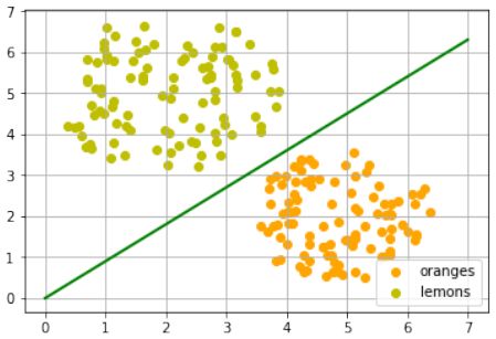
分割线再次是凭肉眼任意设定的。问题是如何系统地做到这一点?我们仍然只关注通过原点的直线,这些直线由其斜率唯一确定。以下 Python 程序通过遍历所有水果并动态调整我们想要计算的分割线的斜率来计算一条分割线。如果一个点在线上方但应该在线下方,斜率将增加
learning_rate的值。如果一个点在线下方但应该在线上方,斜率将减少learning_rate的值。Pythonimport numpy as np import matplotlib.pyplot as plt from itertools import repeat from random import shuffle X = np.arange(0, 8) fig, ax = plt.subplots() # 绘制散点图 ax.scatter(oranges_x, oranges_y, c="orange", label="oranges") ax.scatter(lemons_x, lemons_y, c="y", label="lemons") # 准备数据,为橙子打标签 0,柠檬打标签 1 fruits = list(zip(oranges_x, oranges_y, repeat(0, len(oranges_x)))) fruits += list(zip(lemons_x, lemons_y, repeat(1, len(oranges_x)))) # 修正:这里应该是 len(lemons_x) shuffle(fruits) # 打乱数据 def adjust(learning_rate=0.3, slope=0.3): line = None # 未使用变量 counter = 0 for x, y, label in fruits: res = slope * x - y # 计算点到直线的“距离”(有符号值) #print(label, res) if label == 0 and res < 0: # 如果是橙子 (标签0) 但在线上方 (res < 0) # 点在线上方但应该在下方 # => 增加斜率 slope += learning_rate counter += 1 # ax.plot(X, slope * X, linewidth=2, label=str(counter)) # 每次调整都绘制会很混乱,后续集中绘制 elif label == 1 and res > 0: # 如果是柠檬 (标签1) 但在线下方 (res > 0) # 点在线下方但应该在上方 # => 减少斜率 #print(res, label) slope -= learning_rate counter += 1 # ax.plot(X, slope * X, linewidth=2, label=str(counter)) # 同上 return slope slope = adjust() ax.plot(X, slope * X, linewidth=2, label=f"最终斜率: {slope:.2f}") # 添加标签 ax.legend() ax.grid() plt.show() print(slope)输出会因随机性而异,但类似于:
[<matplotlib.lines.Line2D object at 0x...>]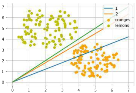
让我们从“柠檬侧”开始使用不同的斜率:
PythonX = np.arange(0, 8) fig, ax = plt.subplots() ax.scatter(oranges_x, oranges_y, c="orange", label="oranges") ax.scatter(lemons_x, lemons_y, c="y", label="lemons") slope = adjust(learning_rate=0.2, slope=3) # 从斜率 3 开始 ax.plot(X, slope * X, linewidth=2, label=f"最终斜率: {slope:.2f}") # 添加标签 ax.legend() ax.grid() plt.show() print(slope)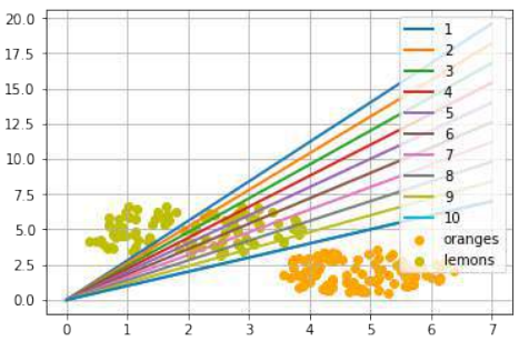
输出会因随机性而异,但类似于:
0.9999999999999996
一个简单的神经网络
我们能够用一条直线将两个类别分开。有人可能会想,这与神经网络有什么关系。我们将在下面阐述这种联系。
我们将定义一个神经网络来分类之前的数据集。我们的神经网络将只包含一个神经元。一个带有两个输入值的神经元,一个用于“酸度”,一个用于“甜度”。
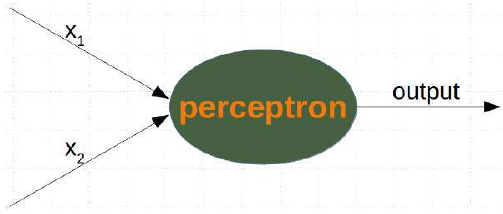
这两个输入值——在下面的 Python 程序中称为
in_data——必须通过权重值进行加权。为了解决我们的问题,我们定义了一个Perceptron类。该类的一个实例就是一个感知器(或神经元)。它可以用input_length(即输入值的数量)和weights(可以作为列表、元组或数组给出)进行初始化。如果没有给出weights的值,或者参数设置为None,我们将把权重初始化为1 / input_length。在下面的例子中,我们选择 -0.45 和 0.5 作为权重值。这不是正常做法。神经网络会在其训练阶段自动计算权重,我们将在后面学习这一点。
Pythonimport numpy as np class Perceptron: def __init__(self, weights): """ 'weights' 可以是一个 numpy 数组、列表或元组,包含权重的实际值。 输入值的数量由 'weights' 的长度间接定义。 """ self.weights = np.array(weights) def __call__(self, in_data): weighted_input = self.weights * in_data weighted_sum = weighted_input.sum() return weighted_sum p = Perceptron(weights=[-0.45, 0.5]) # 使用预设权重 print("橙子结果:") for point in zip(oranges_x[:10], oranges_y[:10]): res = p(point) print(f"{res:.4f}", end=", ") # 格式化输出 print("\n柠檬结果:") for point in zip(lemons_x[:10], lemons_y[:10]): res = p(point) print(f"{res:.4f}", end=", ") # 格式化输出 print()橙子结果: -1.8131, -1.1931, -1.3128, -1.3925, -0.7523, -0.8403, -1.9331, -1.4905, -0.4441, -1.9943, 柠檬结果: 1.9981, 1.1513, 2.5142, 0.4867, 1.7963, 0.8752, 1.5456, 1.6977, 1.4468, 1.4635,我们可以看到,如果我们输入橙子,会得到一个负值;如果我们输入柠檬,会得到一个正值。有了这些知识,我们就可以计算神经网络在这个数据集上的准确性:
Pythonfrom collections import Counter evaluation = Counter() for point in zip(oranges_x, oranges_y): res = p(point) if res < 0: # 橙子期望为负 evaluation['corrects'] += 1 else: evaluation['wrongs'] += 1 for point in zip(lemons_x, lemons_y): res = p(point) if res >= 0: # 柠檬期望为正 evaluation['corrects'] += 1 else: evaluation['wrongs'] += 1 print(evaluation)Counter({'corrects': 200}) # 假设初始生成了 100 个橙子和 100 个柠檬计算是如何进行的?我们将输入值与权重相乘,得到负值和正值。让我们检查一下如果计算结果为 0 会得到什么:
我们可以将这个方程转换为:
我们可以将其与直线的通用形式进行比较:
其中:
-
m 是线的斜率或梯度。
-
c 是线的 y 轴截距。
-
x 是函数的自变量。
我们可以很容易地看到,我们的方程对应于直线的定义,斜率(也称为梯度)m 是
 ,而 c 等于 0。
这是一条分隔橙子和柠檬的直线,被称为决策边界。
我们用以下 Python 程序可视化这一点:
Pythonimport time # 未使用,可以删除 import matplotlib.pyplot as plt import numpy as np # 确保导入 numpy X = np.arange(0, 8) # 修正:X的范围应与数据范围匹配,调整为0到8 fig, ax = plt.subplots() ax.scatter(oranges_x, oranges_y, c="orange", label="oranges") ax.scatter(lemons_x, lemons_y, c="y", label="lemons") # 决策边界的斜率计算 slope = -p.weights[0] / p.weights[1] # slope = 0.45 / 0.5使用感知器 p 的权重 ax.plot(X, slope * X, linewidth=2, label="decision boundary") # 添加标签 ax.grid() ax.legend() # 显示图例 plt.show() print(slope)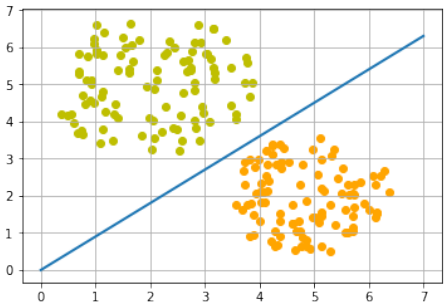
0.9
训练神经网络
正如我们在上一节中提到的:我们没有训练我们的网络。我们调整了权重到我们已知会形成分割线的值。我们现在将演示训练我们简单神经网络所需的东西。
在我们开始这项任务之前,我们将在以下 Python 程序中将我们的数据分成训练数据和测试数据。通过将
random_state设置为 42,我们将获得每次运行相同的输出,这对于调试目的可能很有益。Pythonfrom sklearn.model_selection import train_test_split import random import numpy as np # 确保导入 numpy oranges = list(zip(oranges_x, oranges_y)) # 假设 oranges_x 和 oranges_y 已在之前生成 lemons = list(zip(lemons_x, lemons_y)) # 给橙子打标签 0,柠檬打标签 1: labelled_data = list(zip(oranges + lemons, [0] * len(oranges) + [1] * len(lemons))) random.shuffle(labelled_data) # 打乱数据 data, labels = zip(*labelled_data) # 解包数据和标签 res = train_test_split(data, labels, train_size=0.8, # 80% 作为训练数据 test_size=0.2, # 20% 作为测试数据 random_state=42) # 固定随机种子以保证结果可复现 train_data, test_data, train_labels, test_labels = res print(train_data[:10], train_labels[:10])[(2.592320569178846, 5.623712204925406), (4.7943502284049355, 0.8839613414681706), (2.1239534889189637, 5.377962359316873), (4.130183870483639, 3.2036358839244397), (2.5700607722439957, 3.4894903329620393), (1.1874742907020708, 4.248237496795156), (4.975409937616054, 3.258818001021547), (2.4858113049930375, 3.778544332039814), (0.759896779289841, 4.699741038079466), (1.3275488108562907, 4.204176294559159)] [1, 0, 1, 0, 1, 1, 0, 1, 1, 1]由于我们从两个任意权重开始,我们不能期望结果是正确的。对于某些点(水果),它可能会返回正确的值,即柠檬为 1,橙子为 0。如果我们得到错误的结果,我们必须纠正我们的权重值。首先,我们必须计算误差。误差是目标值或期望值(
target_result)与计算值(calculated_result)之间的差值。有了这个误差,我们必须通过一个增量值来调整权重值,即 。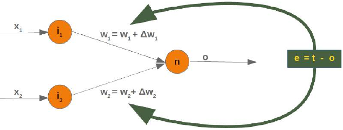
如果误差 e 为 0,即目标结果等于计算结果,我们就不需要做任何事情。对于这些输入值,网络是完美的。如果误差不等于 0,我们必须改变权重。我们必须通过向它们添加小值来改变权重。这些值可以是正的也可以是负的。我们改变权重值的量取决于误差和输入值。假设 x_1 和 x_2 是输入。在这种情况下,结果只取决于输入 x_2。这反过来意味着我们可以通过仅仅改变 w_2 来最小化误差。如果误差是负的,我们将不得不向其添加一个负值;如果误差是正的,我们将不得不向其添加一个正值。由此我们可以理解,无论输入值是什么,我们都可以将它们与误差相乘,然后得到可以添加到权重的值。还有一件事:这样做我们会学得太快。我们有许多样本,每个样本都应该只稍微改变权重。因此,我们必须将这个结果乘以一个学习率(
self.learning_rate)。学习率用于控制权重更新的速度。学习率小会导致训练过程漫长,学习率大则有最终得到次优权重值的风险。我们将在关于反向传播的章节中更详细地了解这一点。我们现在准备编写用于调整权重(即训练网络)的代码。为此,我们在
Perceptron类中添加一个adjust方法。这个方法的任务是纠正误差。Pythonimport numpy as np from collections import Counter class Perceptron: def __init__(self, weights, learning_rate=0.1): """ 'weights' 可以是一个 numpy 数组、列表或元组,包含权重的实际值。 输入值的数量由 'weights' 的长度间接定义。 """ self.weights = np.array(weights) self.learning_rate = learning_rate @staticmethod def unit_step_function(x): if x < 0: return 0 else: return 1 def __call__(self, in_data): weighted_input = self.weights * in_data weighted_sum = weighted_input.sum() #print(in_data, weighted_input, weighted_sum) return Perceptron.unit_step_function(weighted_sum) def adjust(self, target_result, calculated_result, in_data): if not isinstance(in_data, np.ndarray): # 修正:使用 isinstance in_data = np.array(in_data) error = target_result - calculated_result if error != 0: correction = error * in_data * self.learning_rate self.weights += correction #print(target_result, calculated_result, error, in_data, correction, self.weights) def evaluate(self, data, labels): evaluation = Counter() for index in range(len(data)): # 注意:p(data[index]) 返回 0 或 1。round(..., 0) 在这里是多余的。 # int() 转换即可。 label = int(p(data[index])) if label == labels[index]: evaluation["correct"] += 1 else: evaluation["wrong"] += 1 return evaluation p = Perceptron(weights=[0.1, 0.1], # 初始权重 learning_rate=0.3) # 学习率 # 训练感知器 for index in range(len(train_data)): p.adjust(train_labels[index], p(train_data[index]), train_data[index]) # 评估训练数据 evaluation = p.evaluate(train_data, train_labels) print(evaluation.most_common()) # 评估测试数据 evaluation = p.evaluate(test_data, test_labels) print(evaluation.most_common()) print(p.weights)[('correct', 160)] [('correct', 40)] [-1.68135341 2.07512397]无论是学习数据还是测试数据,我们都只有正确的值,这意味着我们的网络能够自动且成功地学习!
我们用以下程序可视化决策边界:
Pythonimport matplotlib.pyplot as plt import numpy as np X = np.arange(0, 7) # 绘制直线的 X 范围 fig, ax = plt.subplots() # 从训练数据中分离柠檬和橙子,以便可视化 lemons = [train_data[i] for i in range(len(train_data)) if train_labels[i] == 1] lemons_x, lemons_y = zip(*lemons) oranges = [train_data[i] for i in range(len(train_data)) if train_labels[i] == 0] oranges_x, oranges_y = zip(*oranges) ax.scatter(oranges_x, oranges_y, c="orange", label="Oranges") # 添加标签 ax.scatter(lemons_x, lemons_y, c="y", label="Lemons") # 添加标签 w1 = p.weights[0] w2 = p.weights[1] m = -w1 / w2 # 计算决策边界的斜率 ax.plot(X, m * X, label="Decision Boundary", color="g", linewidth=2) # 绘制决策边界,增加颜色和线宽 ax.legend() # 显示图例 plt.show() print(p.weights)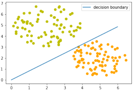
[-1.68135341 2.07512397]让我们来看看算法“运动”起来的样子。
Pythonimport numpy as np import matplotlib.pyplot as plt import matplotlib.cm as cm # 导入颜色映射模块 p = Perceptron(weights=[0.1, 0.1], # 初始权重 learning_rate=0.3) # 学习率 number_of_colors = 7 colors = cm.rainbow(np.linspace(0, 1, number_of_colors)) # 生成彩虹色系 fig, ax = plt.subplots() ax.set_xticks(range(8)) # 设置 X 轴刻度 ax.set_ylim([-2, 8]) # 设置 Y 轴范围 counter = 0 for index in range(len(train_data)): old_weights = p.weights.copy() # 复制旧权重以检查是否发生变化 p.adjust(train_labels[index], p(train_data[index]), train_data[index]) if not np.array_equal(old_weights, p.weights): # 如果权重发生了变化 color = "orange" if train_labels[index] == 0 else "y" # 根据标签选择颜色 ax.scatter(train_data[index][0], train_data[index][1], color=color) ax.annotate(str(counter), # 标记改变权重的点 (train_data[index][0], train_data[index][1]), textcoords="offset points", xytext=(0,10), ha='center') # 调整标注位置 m = -p.weights[0] / p.weights[1] # 计算新的决策边界斜率 print(index, f"{m:.4f}", p.weights, train_data[index]) # 打印当前索引、斜率、权重和数据点 ax.plot(X, m * X, label=f"Line {counter}", color=colors[counter % number_of_colors], linewidth=1) # 绘制决策边界并添加标签 counter += 1 ax.legend() # 显示图例 plt.show()1 -3.0400 [-1.45643048 -0.4790835 ] (5.188101611742407, 1.930278325463612) 2 0.5906 [-0.73406347 1.24291557] (2.4078900359381787, 5.739996893315745) 18 6.7005 [-2.03694068 0.30399756] (4.342924008657758, 3.129726697580847) 20 0.5044 [-0.87357998 1.73188666] (3.877868972161467, 4.759630340827767) 27 2.7419 [-2.39560903 0.87370868] (5.073430165416017, 2.8605932860372967) 31 0.8102 [-1.68135341 2.07512397] (2.38085207252672, 4.004717642222739)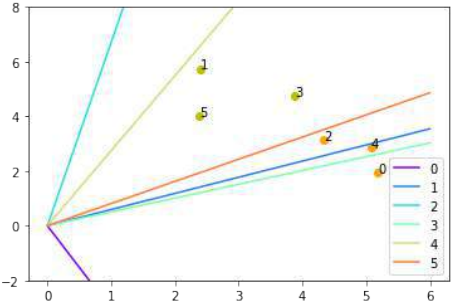
图中每个点都会引起权重的变化。我们按照它们出现的顺序给它们编号,并显示相应的直线。通过这种方式,我们可以看到网络是如何“学习”的。
We will develop a simple neural network in this chapter of our tutorial. A network capable of separating two
classes, which are separable by a straight line in a 2-dimensional feature space.
LINE SEPARATION
Before we start programming a simple neural
network, we are going to develop a different concept.
We want to search for straight lines that separate two
points or two classes in a plane. We will only look at
straight lines going through the origin. We will look
at general straight lines later in the tutorial.
You could imagine that you have two attributes
describing an eddible object like a fruit for example:
"sweetness" and "sourness".
We could describe this by points in a two-
dimensional space. The A axis is used for the values
of sweetness and the y axis is correspondingly used
for the sourness values. Imagine now that we have
two fruits as points in this space, i.e. an orange at
position (3.5, 1.8) and a lemon at (1.1, 3.9).
We could define dividing lines to define the points which are more lemon-like and which are more orange-
like.
In the following diagram, we depict one lemon and one orange. The green line is separating both points. We
assume that all other lemons are above this line and all oranges will be below this line.
96
The green line is defined by
y = mx
where:
m is the slope or gradient of the line and x is the independent variable of the function.
p2
m =
x
p 1
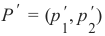
This means that a point P ′ = (p ′ , p ′ ) is on this line, if the following condition is fulfilled:
1
2
mp ′ − p ′ = 0
1
2
The following Python program plots a graph depicting the previously described situation:
import matplotlib.pyplot as plt
import numpy as np
97
X = np.arange(0, 7)
fig, ax = plt.subplots()
ax.plot(3.5, 1.8, "or",
color="darkorange",
markersize=15)
ax.plot(1.1, 3.9, "oy",
markersize=15)
point_on_line = (4, 4.5)
ax.plot(1.1, 3.9, "oy", markersize=15)
# calculate gradient:
m = point_on_line[1] / point_on_line[0]
ax.plot(X, m * X, "g-", linewidth=3)
plt.show()
It is clear that a point A = (a 1, a 2) is not on the line, if m ⋅ a 1 − a 2 is not equal to 0. We want to know more.
We want to know, if a point is above or below a straight line.
98
If a point B = (b 1, b 2) is below this line, there must be a δ B > 0 so that the point (b1, b 2 + δB) will be on the
line.
This means that
m ⋅ b1 − (b2 + δ B) = 0
which can be rearranged to
m ⋅ b 1 − b 2 = δB
Finally, we have a criteria for a point to be below the line. m ⋅ b 1 − b2 is positve, because δ B is positive.
The reasoning for "a point is above the line" is analogue: If a point A = (a1, a 2) is above the line, there must
be a δA > 0 so that the point (a1, a 2 − δ A) will be on the line.
This means that
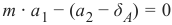
m ⋅ a1 − (a2 − δ A) = 0
which can be rearranged to
m ⋅ a 1 − a2 = − δ A
99
In summary, we can say: A point P(p1, p 2) lies
•••below the straight line if m ⋅ p 1 − p 2 > 0
on the straight line if m ⋅ p 1 − p 2 = 0
above the straight line if m ⋅ p 1 − p 2 < 0
We can now verify this on our fruits. The lemon has the coordinates (1.1, 3.9) and the orange the coordinates
3.5, 1.8. The point on the line, which we used to define our separation straight line has the values (4, 4.5). So
m is 4.5 divides by 4.
lemon = (1.1, 3.9)
orange = (3.5, 1.8)
m = 4.5 / 4
# check if orange is below the line,
# positive value is expected:
print(orange[0] * m - orange[1])
# check if lemon is above the line,
# negative value is expected:
print(lemon[0] * m - lemon[1])
2.1375
-2.6624999999999996
We did not calculate the green line using mathematical formulas or methods, but arbitrarily determined it by
visual judgement. We could have chosen other lines as well.
The following Python program calculates and renders a bunch of lines. All going through the origin, i.e. the
point (0, 0). The red ones are completely unusable for the purpose of separating the two fruits, because in
these cases both the lemon and the orange are on the same side of the straight line. However, it is obvious that
even the green ones might not be too useful if we have more than these two fruits. Some lemons might be
sweeter and some oranges can be quite sour.
import numpy as np
import matplotlib.pyplot as plt
def create_distance_function(a, b, c):
""" 0 = ax + by + c """
def distance(x, y):
"""
returns tuple (d, pos)
d is the distance
100
If pos == -1 point is below the line,
0 on the line and +1 if above the line
"""
nom = a * x + b * y + c
if nom == 0:
pos = 0
elif (nom<0 and b<0) or (nom>0 and b>0):
pos = -1
else:
pos = 1
return (np.absolute(nom) / np.sqrt( a ** 2 + b ** 2),return distance
orange = (4.5, 1.8)
lemon = (1.1, 3.9)
fruits_coords = [orange, lemon]
fig, ax = plt.subplots()
ax.set_xlabel("sweetness")
ax.set_ylabel("sourness")
x_min, x_max = -1, 7
y_min, y_max = -1, 8
ax.set_xlim([x_min, x_max])
ax.set_ylim([y_min, y_max])
X = np.arange(x_min, x_max, 0.1)
step = 0.05
for x in np.arange(0, 1+step, step):
slope = np.tan(np.arccos(x))
dist4line1 = create_distance_function(slope, -1, 0)
Y = slope * X
results = []
for point in fruits_coords:
results.append(dist4line1(*point))
if (results[0][1] != results[1][1]):
ax.plot(X, Y, "g-", linewidth=0.8, alpha=0.9)
else:
ax.plot(X, Y, "r-", linewidth=0.8, alpha=0.9)
size = 10
for (index, (x, y)) in enumerate(fruits_coords):
if index== 0:
ax.plot(x, y, "o",
color="darkorange",
markersize=size)
pos)
101
else:
ax.plot(x, y, "oy",
markersize=size)
plt.show()
Basically, we have carried out a classification based on our dividing line. Even if hardly anyone would
describe this as such.
It is easy to imagine that we have more lemons and oranges with slightly different sourness and sweetness
values. This means we have a class of lemons ( class1 ) and a class of oranges class2 . This is depicted
in the following diagram.
102
We are going to "grow" oranges and lemons with a Python program. We will create these two classes by
randomly creating points within a circle with a defined center point and radius. The following Python code
will create the classes:
import numpy as np
import matplotlib.pyplot as plt
def points_within_circle(radius,
center=(0, 0),
number_of_points=100):
center_x, center_y = center
r = radius * np.sqrt(np.random.random((number_of_points,)))
theta = np.random.random((number_of_points,)) * 2 * np.pi
x = center_x + r * np.cos(theta)
y = center_y + r * np.sin(theta)
return x, y
X = np.arange(0, 8)
fig, ax = plt.subplots()
oranges_x, oranges_y = points_within_circle(1.6, (5, 2), 100)
lemons_x, lemons_y = points_within_circle(1.9, (2, 5), 100)
ax.scatter(oranges_x,
oranges_y,
c="orange",
label="oranges")
ax.scatter(lemons_x,
103
lemons_y,
c="y",
label="lemons")
ax.plot(X, 0.9 * X, "g-", linewidth=2)
ax.legend()
ax.grid()
plt.show()
The dividing line was again arbitrarily set by eye. The question arises how to do this systematically? We are
still only looking at straight lines going through the origin, which are uniquely defined by its slope. the
following Python program calculates a dividing line by going through all the fruits and dynamically adjusts
the slope of the dividing line we want to calculate. If a point is above the line but should be below the line, the
slope will be increment by the value of learning_rate . If the point is below the line but should be above
the line, the slope will be decremented by the value of learning_rate .
import numpy as np
import matplotlib.pyplot as plt
from itertools import repeat
from random import shuffle
X = np.arange(0, 8)
fig, ax = plt.subplots()
ax.scatter(oranges_x,
oranges_y,
c="orange",
label="oranges")
ax.scatter(lemons_x,
104
lemons_y,
c="y",
label="lemons")
fruits = list(zip(oranges_x,
oranges_y,
repeat(0, len(oranges_x))))
fruits += list(zip(lemons_x,
lemons_y,
repeat(1, len(oranges_x))))
shuffle(fruits)
def adjust(learning_rate=0.3, slope=0.3):
line = None
counter = 0
for x, y, label in fruits:
res = slope * x - y
#print(label, res)
if label == 0 and res < 0:
# point is above line but should be below
# => increment slope
slope += learning_rate
counter += 1
ax.plot(X, slope * X,
linewidth=2, label=str(counter))
elif label == 1 and res > 0:
# point is below line but should be above
# => decrement slope
#print(res, label)
slope -= learning_rate
counter += 1
ax.plot(X, slope * X,
linewidth=2, label=str(counter))
return slope
slope = adjust()
ax.plot(X,
slope * X,
linewidth=2)
ax.legend()
ax.grid()
plt.show()
105
print(slope)
[<matplotlib.lines.Line2D object at 0x7f53b0a22c50>]
Let's start with a different slope from the 'lemon side':
X = np.arange(0, 8)
fig, ax = plt.subplots()
ax.scatter(oranges_x,
oranges_y,
c="orange",
label="oranges")
ax.scatter(lemons_x,
lemons_y,
c="y",
label="lemons")
slope = adjust(learning_rate=0.2, slope=3)
ax.plot(X,
slope * X,
linewidth=2)
ax.legend()
ax.grid()
plt.show()
print(slope)
106
0.9999999999999996
A SIMPLE NEURAL NETWORK
We were capable of separating the two classes with a straight line. One might wonder what this has to do with
neural networks. We will work out this connection below.
We are going to define a neural network to classify the previous data sets. Our neural network will only
consist of one neuron. A neuron with two input values, one for 'sourness' and one for 'sweetness'.
The two input values - called in_data in our Python program below - have to be weighted by weight
values. So solve our problem, we define a Perceptron class. An instance of the class is a Perceptron (or
Neuron). It can be initialized with the input_length, i.e. the number of input values, and the weights, which can
be given as a list, tuple or an array. If there are no values for the weights given or the parameter is set to None,
we will initialize the weights to 1 / input_length.
In the following example choose -0.45 and 0.5 as the values for the weights. This is not the normal way to do
it. A Neural Network calculates the weights automatically during its training phase, as we will learn later.
import numpy as np
107
class Perceptron:
def __init__(self, weights):
"""
'weights' can be a numpy array, list or a tuple with the
actual values of the weights. The number of input values
is indirectly defined by the length of 'weights'
"""
self.weights = np.array(weights)
def __call__(self, in_data):
weighted_input = self.weights * in_data
weighted_sum = weighted_input.sum()
return weighted_sum
p = Perceptron(weights=[-0.45, 0.5])
for point in zip(oranges_x[:10], oranges_y[:10]):
res = p(point)
print(res, end=", ")
for point in zip(lemons_x[:10], lemons_y[:10]):
res = p(point)
print(res, end=", ")
-1.8131460150609238, -1.1931285955719209, -1.3127632381850327,
-1.3925163810790897, -0.7522874009031233, -0.8402958901009828,
-1.9330506389030604, -1.490534974734101, -0.4441170096959772, -1.9
942817372340516, 1.998076257605724, 1.1512784858148413, 2.51418870
799987, 0.4867012212497872, 1.7962680593822624, 0.875162742271260
9, 1.5455925862569528, 1.6976576197574347, 1.4467637066140102, 1.4
634541513290587,
We can see that we get a negative value, if we input an orange and a posive value, if we input a lemon. With
this knowledge, we can calculate the accuracy of our neural network on this data set:
from collections import Counter
evaluation = Counter()
for point in zip(oranges_x, oranges_y):
res = p(point)
if res < 0:
evaluation['corrects'] += 1
else:
evaluation['wrongs'] += 1
108
for point in zip(lemons_x, lemons_y):
res = p(point)
if res >= 0:
evaluation['corrects'] += 1
else:
evaluation['wrongs'] += 1
print(evaluation)
Counter({'corrects':200})
How does the calculation work? We multiply the input values with the weights and get negative and positive
values. Let us examine what we get, if the calculation results in 0:
w 1 ⋅ x 1 + w 2 ⋅ x 2 = 0
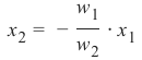
We can change this equation into
w1
x2 = −
⋅ x 1
w2
We can compare this with the general form of a straight line
y = m ⋅ x + c
where:
• m is the slope or gradient of the line.
• c is the y-intercept of the line.
• x is the independent variable of the function.
We can easily see that our equation corresponds to the definition of a line and the slope (aka gradient) m is
w1
− and c is equal to 0.
w2
This is a straight line separating the oranges and lemons, which is called the decision boundary.
We visualize this with the following Python program:
import time
import matplotlib.pyplot as plt
slope = 0.1
X = np.arange(0, 8)
109
fig, ax = plt.subplots()
ax.scatter(oranges_x,
oranges_y,
c="orange",
label="oranges")
ax.scatter(lemons_x,
lemons_y,
c="y",
label="lemons")
slope = 0.45 / 0.5
ax.plot(X, slope * X,
linewidth=2)
ax.grid()
plt.show()
print(slope)
0.9
TRAINING A NEURAL NETWORK
As we mentioned in the previous section: We didn't train our network. We have adjusted the weights to values
that we know would form a dividing line. We want to demonstrate now, what is necessary to train our simple
neural network.
Before we start with this task, we will separate our data into training and test data in the following Python
program. By setting the random_state to the value 42 we will have the same output for every run, which can
be benifial for debugging purposes.
110
from sklearn.model_selection import train_test_split
import random
oranges = list(zip(oranges_x, oranges_y))
lemons = list(zip(lemons_x, lemons_y))
# labelling oranges with 0 and lemons with 1:
labelled_data = list(zip(oranges + lemons,
[0] * len(oranges) + [1] * len(lemons)))
random.shuffle(labelled_data)
data, labels = zip(*labelled_data)
res = train_test_split(data, labels,
train_size=0.8,
test_size=0.2,
random_state=42)
train_data, test_data, train_labels, test_labels = res
print(train_data[:10], train_labels[:10])
[(2.592320569178846, 5.623712204925406), (4.7943502284049355, 0.88
39613414681706), (2.1239534889189637, 5.377962359316873), (4.13018
3870483639, 3.2036358839244397), (2.5700607722439957, 3.4894903329
620393), (1.1874742907020708, 4.248237496795156), (4.9754099376160
54, 3.258818001021547), (2.4858113049930375, 3.778544332039814),
(0.759896779289841, 4.699741038079466), (1.3275488108562907, 4.204
176294559159)] [1, 0, 1, 0, 1, 1, 0, 1, 1, 1]
As we start with two arbitrary weights, we cannot expect the result to be correct. For some points (fruits) it
may return the proper value, i.e. 1 for a lemon and 0 for an orange. In case we get the wrong result, we have to
correct our weight values. First we have to calculate the error. The error is the difference between the target or
expected value ( target_result ) and the calculated value ( calculated_result ). With this error
we have to adjust the weight values with an incremental value, i.e. w1 = w 1 + Δw 1 and w2 = w 2 + Δw 2
111
If the error e is 0, i.e. the target result is equal to the calculated result, we don't have to do anything. The
network is perfect for these input values. If the error is not equal, we have to change the weights. We have to
change the weights by adding small values to them. These values may be positive or negative. The amount we
have a change a weight value depends on the error and on the input value. Let us assume, x = 0 and x > 0.
1 2In this case the result in this case solely results on the input x 2. This on the other hand means that we can
minimize the error by changing solely w 2. If the error is negative, we will have to add a negative value to it,
and if the error is positive, we will have to add a positive value to it. From this we can understand that
whatever the input values are, we can multiply them with the error and we get values, we can add to the
weights. One thing is still missing: Doing this we would learn to fast. We have many samples and each sample
should only change the weights a little bit. Therefore we have to multiply this result with a learning rate
( self.learning_rate ). The learning rate is used to control how fast the weights are updated. Small
values for the learning rate result in a long training process, larger values bear the risk of ending up in sub-
optimal weight values. We will have a closer look at this in our chapter on backpropagation.
We are ready now to write the code for adapting the weights, which means training the network. For this
purpose, we add a method 'adjust' to our Perceptron class. The task of this method is to crrect the error.
import numpy as np
from collections import Counter
class Perceptron:
def __init__(self,
weights,
learning_rate=0.1):
"""
'weights' can be a numpy array, list or a tuple with the
actual values of the weights. The number of input values
is indirectly defined by the length of 'weights'
"""
self.weights = np.array(weights)
self.learning_rate = learning_rate
@staticmethod
def unit_step_function(x):
if x < 0:
return 0
else:
return 1
def __call__(self, in_data):
weighted_input = self.weights * in_data
weighted_sum = weighted_input.sum()
#print(in_data, weighted_input, weighted_sum)
112
return Perceptron.unit_step_function(weighted_sum)
def adjust(self,
target_result,
calculated_result,
in_data):
if type(in_data) != np.ndarray:
in_data = np.array(in_data) #
error = target_result - calculated_result
if error != 0:
correction = error * in_data * self.learning_rate
self.weights += correction
#print(target_result, calculated_result, error, in_dat
a, correction, self.weights)
def evaluate(self, data, labels):
evaluation = Counter()
for index in range(len(data)):
label = int(round(p(data[index]),0))
if label == labels[index]:
evaluation["correct"] += 1
else:
evaluation["wrong"] += 1
return evaluation
p = Perceptron(weights=[0.1, 0.1],
learning_rate=0.3)
for index in range(len(train_data)):
p.adjust(train_labels[index],
p(train_data[index]),
train_data[index])
evaluation = p.evaluate(train_data, train_labels)
print(evaluation.most_common())
evaluation = p.evaluate(test_data, test_labels)
print(evaluation.most_common())
print(p.weights)
[('correct',[('correct',[-1.68135341160)]
40)]
2.07512397]
113
Both on the learning and on the test data, we have only correct values, i.e. our network was capable of learning
automatically and successfully!
We visualize the decision boundary with the following program:
import matplotlib.pyplot as plt
import numpy as np
X = np.arange(0, 7)
fig, ax = plt.subplots()
lemons = [train_data[i] for i in range(len(train_data)) if train_l
abels[i] == 1]
lemons_x, lemons_y = zip(*lemons)
oranges = [train_data[i] for i in range(len(train_data)) if trai
n_labels[i] == 0]
oranges_x, oranges_y = zip(*oranges)
ax.scatter(oranges_x, oranges_y, c="orange")
ax.scatter(lemons_x, lemons_y, c="y")
w1 = p.weights[0]
w2 = p.weights[1]
m = -w1 / w2
ax.plot(X, m * X, label="decision boundary")
ax.legend()
plt.show()
print(p.weights)
[-1.68135341
2.07512397]
114
Let us have a look on the algorithm "in motion".
import numpy as np
import matplotlib.pyplot as plt
import matplotlib.cm as cm
p = Perceptron(weights=[0.1, 0.1],
learning_rate=0.3)
number_of_colors = 7
colors = cm.rainbow(np.linspace(0, 1, number_of_colors))
fig, ax = plt.subplots()
ax.set_xticks(range(8))
ax.set_ylim([-2, 8])
counter = 0
for index in range(len(train_data)):
old_weights = p.weights.copy()
p.adjust(train_labels[index],
p(train_data[index]),
train_data[index])
if not np.array_equal(old_weights, p.weights):
color = "orange" if train_labels[index] == 0 else
"y"
ax.scatter(train_data[index][0],
train_data[index][1],
color=color)
ax.annotate(str(counter),
(train_data[index][0], train_data[index][1]))
m = -p.weights[0] / p.weights[1]
print(index, m, p.weights, train_data[index])
ax.plot(X, m * X, label=str(counter), color=colors[counte
r])
counter += 1
ax.legend()
plt.show()
115
1 -3.0400347553192493 [-1.45643048 -0.4790835 ] (5.18810161174240
7, 1.930278325463612)
2 0.5905980182798966 [-0.73406347 1.24291557] (2.407890035938178
7, 5.739996893315745)
18 6.70051650445074 [-2.03694068 0.30399756] (4.342924008657758,
3.129726697580847)
20 0.5044094409795936 [-0.87357998 1.73188666] (3.87786897216146
7, 4.759630340827767)
27 2.7418853617419434 [-2.39560903 0.87370868] (5.07343016541601
7, 2.8605932860372967)
31 0.8102423930878537 [-1.68135341 2.07512397] (2.3808520725267
2, 4.004717642222739)
Each of the points in the diagram above cause a change in the weights. We see them numbered in the order of
their appearance and the corresponding straight line. This way we can see how the networks "learns". -